<?xml version="1.0" encoding="utf-8"?><feed xmlns="http://www.w3.org/2005/Atom" ><generator uri="https://jekyllrb.com/" version="3.10.0">Jekyll</generator><link href="https://joelholder.com/feed.xml" rel="self" type="application/atom+xml" /><link href="https://joelholder.com/" rel="alternate" type="text/html" /><updated>2026-08-05T00:05:46+00:00</updated><id>https://joelholder.com/feed.xml</id><title type="html">Joel Holder</title><subtitle>Math, coding, philosophy, art, and other things that interest me</subtitle><author><name>Joel Holder</name></author><entry><title type="html">The Staircase and the Slide</title><link href="https://joelholder.com/blog/2026/07/21/the-staircase-and-the-slide/" rel="alternate" type="text/html" title="The Staircase and the Slide" /><published>2026-07-21T05:10:00+00:00</published><updated>2026-07-21T05:10:00+00:00</updated><id>https://joelholder.com/blog/2026/07/21/the-staircase-and-the-slide</id><content type="html" xml:base="https://joelholder.com/blog/2026/07/21/the-staircase-and-the-slide/"><![CDATA[<style>
.staircase-post .katex-display > .katex { font-size: 1.35em !important; }
.staircase-post .katex { font-size: 1.3em !important; }
</style>

<div class="staircase-post">

  <p>A staircase and a ramp can connect the same two floors. Stand at the bottom of each and they look like different ideas entirely — one moves in flat steps and sudden jumps, the other in one continuous rise. Digital and analog. Pixels and ink. A number line marked only at the integers, versus a number line with no gaps in it anywhere.</p>

  <p>Discreteness counts. Continuity flows. They feel like two different worlds.</p>

  <p>This post is about a place where those two worlds turn out to be the same picture, seen at two different resolutions. We won’t name where we’re headed just yet — better to let it arrive on its own.</p>

  <h2 id="quick-recap-the-staircase-we-already-built">Quick recap: the staircase we already built</h2>

  <p><a href="/blog/2026/07/12/gauss-pascal-and-triangular-numbers/">Last time</a>, we stacked blocks in rows — 1 block, then 2, then 3, and so on — and asked how many blocks were in the whole triangular stack.</p>

  <p>Let’s fix the names we’ll reuse throughout this post:</p>

  <ul>
    <li>$n$ is how many rows we stack — how far we count up to.</li>
    <li>$T(n)$ is the total number of blocks once we’ve stacked all $n$ rows.</li>
  </ul>

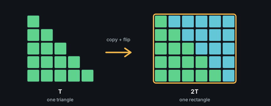
  <p>We found $T(n)$ by copying the stack, flipping the copy upside down, and fitting the two together into a plain rectangle:</p>

  <figure class="math-figure">
  <img src="/assets/math/gauss-pascal-triangular/triangle-rectangle-proof.svg" alt="A five-row triangular stack of blocks copied and flipped to form a five by six rectangle" />
  <figcaption>The triangular numbers, one more time: a stack of blocks is exactly half of a rectangle.</figcaption>
</figure>

  <p>A rectangle is easy: it’s just rows times columns, cut in half to undo the copy:</p>

\[T(n) = \dfrac{n(n + 1)}{2}\]

  <p>That’s where we left off. Now we’re going to take that same staircase and start shrinking its steps.</p>

  <h2 id="a-series-is-just-a-sum-one-term-at-a-time">A series is just a sum, one term at a time</h2>

  <p>Let’s slow down and name a couple of things carefully before we go further.</p>

  <p>A <strong>sequence</strong> is nothing more than a list of numbers, in order: $1, 2, 3, 4, 5, \dots$ That’s it. No trick to it.</p>

  <p>A <strong>series</strong> takes a sequence and starts adding its terms together, one at a time. If you stop after some number of terms, what you get is called a <strong>partial sum</strong> — the running total up to that point.</p>

  <p>That’s exactly what $T(n)$ has been the whole time, we just didn’t use these words for it yet. $T(n)$ <em>is</em> the partial sum of the sequence of counting numbers, stopped after $n$ terms:</p>

\[T(n) = 1 + 2 + 3 + \cdots + n\]

  <p>Nothing new has happened here. We’re only putting a name on something we’ve already been doing since the last post.</p>

  <h2 id="watching-the-sum-grow-one-step-at-a-time">Watching the sum grow, one step at a time</h2>

  <p>Now let’s watch what happens to that running total as one more term joins it. Two concrete partial sums, side by side:</p>

\[T(4) = 1+2+3+4 = 10 \qquad\qquad T(5) = 1+2+3+4+5 = 15\]

  <p>Compare them:</p>

\[T(5) - T(4) = 15 - 10 = 5\]

  <p>That’s not a coincidence, and it’s not special to 4 and 5. $T(5)$ is just $T(4)$ with one new term tacked on — the term $5$ itself. Of course the difference is $5$. In general, going from $n-1$ terms to $n$ terms adds exactly one new term, and that new term is $n$:</p>

\[T(n) - T(n-1) = n\]

  <p>Hang on to that. <strong>Every time $n$ goes up by one, $T(n)$ goes up by exactly $n$.</strong></p>

  <h2 id="difference-quotients-and-a-staircase-where-h--1">Difference quotients, and a staircase where h = 1</h2>

  <p>We just found something true specifically about $T$: it grows by exactly $n$ every time $n$ increases by 1. Before we go further, it’s worth learning the general version of what we just did — the version that works for <em>any</em> function, not just $T$ — because we’re about to reuse it on shapes and areas, too.</p>

  <p>Here’s the general setup, with no staircase in it yet. Take any function $f$. Pick some input to start from, and call it $a$ — just a placeholder name for “wherever we happen to be starting.” Now take a step: move the input away from $a$ by some amount, and call the size of that step $h$. Moving the input by $h$ takes us from $a$ to $a+h$, and the function’s output moves too — from $f(a)$ to $f(a+h)$.</p>

  <p>Two new letters, both doing simple jobs: $a$ names the starting point, and $h$ names how big a step we took away from it. Neither one is tied to any particular function or number yet — they’re placeholders that work the same way no matter what $f$ happens to be.</p>

  <p>With that fully in view, here’s the definition. The quantity</p>

\[\dfrac{f(a+h) - f(a)}{h}\]

  <p>is called a <strong>difference quotient</strong>. Read the pieces separately: $f(a+h)$ is the function’s value after the step, $f(a)$ is its value before the step, so $f(a+h) - f(a)$ is how much $f$ changed. Dividing by $h$ turns that change into a rate — change <em>per unit of input</em>, over a step of size $h$.</p>

  <p>Now let’s connect this back to the staircase. Our function is $T$. A moment ago, we moved from $T(n-1)$ to $T(n)$ — in the language we just built, that’s starting point $a = n-1$, and step size $h = 1$, since the input moved from $n-1$ to $n$, a jump of exactly one unit. That’s the only step size we’ll use for most of this post: $h=1$, always, because we’re only ever moving from one whole number to the very next one. Later on, we’ll deliberately let $h$ shrink smaller than 1 — but not yet.</p>

  <p>Apply the difference quotient to $T$, with $a = n-1$ and $h=1$:</p>

\[\dfrac{T(n) - T(n-1)}{h} = \dfrac{T(n)-T(n-1)}{1} = T(n) - T(n-1)\]

  <p>Dividing by $h=1$ doesn’t change anything — so the difference quotient of $T$ is just the plain difference we already found by hand a moment ago: $n$. Rearranged, that’s the relationship we’ll lean on for the rest of this post:</p>

\[T(n) = T(n-1) + n\]

  <h2 id="the-staircase-is-a-rough-sketch-of-a-line">The staircase is a rough sketch of a line</h2>

  <p>Picture the blocks again, but as bars: a bar of height 1, then height 2, then 3, up to height $n$. We just showed that each bar adds exactly the next counting number to the running total — a difference quotient of $n$, with $h=1$.</p>

  <p>That “$+n$” is worth sitting with. The bars aren’t growing by some rule bolted on from outside. They grow by exactly the next whole number, because whole numbers are spaced exactly 1 apart. The staircase has no choice but to look like this — it’s the number line, stood up in blocks.</p>

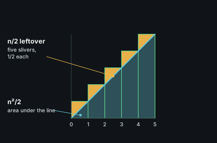
  <p>Now draw the line $y = x$ underneath the bars.</p>

  <figure class="math-figure">
  <img src="/assets/math/staircase-to-integral/staircase-overshoot.svg" alt="Five bars of increasing height sitting above the diagonal line y equals x, with the overshoot triangles shaded" />
  <figcaption>Each bar overshoots the line by a small triangular sliver — always the same size.</figcaption>
</figure>

  <p>The bars hug that line closely, but not perfectly. Each bar sits a little taller than the line beneath it, everywhere except at its top-right corner, where the two touch.</p>

  <p>The gap between a bar’s flat top and the line rising underneath it is a little right triangle. Every one of those triangles has legs of length 1 — the width of a bar, and the amount the line climbs across that width. Legs of 1 and 1 mean area $\dfrac{1}{2}$, every time, no matter how tall the bar is.</p>

  <h2 id="where-the-line-was-hiding">Where the line was hiding</h2>

  <p>So the staircase is really two things stacked together: the region under the line, plus $n$ identical leftover slivers of area $\dfrac{1}{2}$.</p>

  <p>Why talk about <em>area</em> at all, though? Last time, we counted blocks by stacking them, and since each block has area 1, counting blocks <em>was</em> computing area, in block-units. Nothing about that has changed. Each bar has width $h$, and right now $h=1$, so a bar of height $k$ still covers exactly $k$ square units — the same $k$ we were always adding. Summing bar areas is just another way of writing $T(n)$. It always was.</p>

  <p>Let’s find those two areas, step by step, without skipping anything.</p>

  <p><strong>The region under the line.</strong> It’s a right triangle with base $n$ and height $n$, since the line runs from $(0,0)$ to $(n,n)$.</p>

  <div class="proof-sequence">
    <div class="proof-step">
      <p><strong>The rectangle around it</strong></p>

      <p class="step-formula">\(n \times n = n^2\)</p>
    </div>

    <div class="proof-step">
      <p><strong>The triangle is half that rectangle</strong></p>

      <p class="step-formula">\(\dfrac{n^2}{2}\)</p>
    </div>
  </div>

  <p>Same halving move as the two-triangles-make-a-rectangle picture from last time — just applied to a slope instead of a stack of blocks.</p>

  <p><strong>The leftover slivers.</strong> Each one is a right triangle whose legs both equal $h$, and $h=1$ here.</p>

  <div class="proof-sequence">
    <div class="proof-step">
      <p><strong>One sliver’s legs</strong></p>

      <p class="step-formula">\(h = 1, \quad h = 1\)</p>
    </div>

    <div class="proof-step">
      <p><strong>One sliver’s area</strong></p>

      <p class="step-formula">\(\dfrac{h \times h}{2} = \dfrac{1 \times 1}{2} = \dfrac{1}{2}\)</p>
    </div>

    <div class="proof-step">
      <p><strong>All $n$ slivers together</strong></p>

      <p class="step-formula">\(n \times \dfrac{1}{2} = \dfrac{n}{2}\)</p>
    </div>
  </div>

  <p>Now watch what happens when we split the formula we already had:</p>

  <div class="proof-sequence">
    <div class="proof-step">
      <p><strong>Start from what we proved last time</strong></p>

      <p class="step-formula">\(T(n) = \dfrac{n(n+1)}{2}\)</p>
    </div>

    <div class="proof-step">
      <p><strong>Expand the numerator</strong></p>

      <p class="step-formula">\(T(n) = \dfrac{n^2 + n}{2}\)</p>
    </div>

    <div class="proof-step">
      <p><strong>Split the fraction</strong></p>

      <p class="step-formula">\(T(n) = \dfrac{n^2}{2} + \dfrac{n}{2}\)</p>
    </div>
  </div>

  <p>That split isn’t a trick of algebra. It’s the picture, in symbols. $\dfrac{n^2}{2}$ is the smooth triangle under the line — the one we just found by halving a rectangle. $\dfrac{n}{2}$ is the pile of leftover slivers — the one we just found by adding up $n$ little half-square triangles. Same two areas, twice now: once from the picture, once from the algebra.</p>

  <p>Let’s slow down and check that against actual numbers — the same five bars pictured above, where $n = 5$.</p>

  <p>First, the formula from last time, plugged in directly:</p>

\[T(5) = \dfrac{5 \cdot 6}{2} = \dfrac{30}{2} = 15\]

  <p>Now split that 15 the same way we just split $T(n)$ in general:</p>

\[T(5) = \dfrac{5^2}{2} + \dfrac{5}{2} = \dfrac{25}{2} + \dfrac{5}{2} = 12.5 + 2.5\]

  <p>$12.5$ is the smooth triangle — five columns wide, five tall, cut in half. $2.5$ is the five little slivers, $\dfrac{1}{2}$ each, one riding on top of every bar. Add the two pieces back together and we’re at 15 again, exactly where we started:</p>

\[12.5 + 2.5 = 15\]

  <h2 id="shrinking-the-grain">Shrinking the grain</h2>

  <p>Natural next question: what if the steps were narrower?</p>

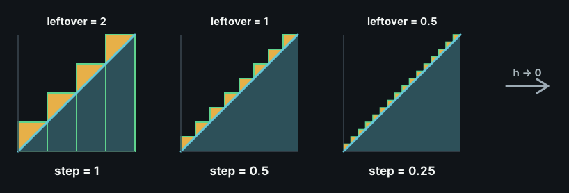
  <p>Use bars of width $h$ instead of width 1 — a half, a quarter, anything smaller. Rebuild the same staircase over the same line, out of finer steps.</p>

  <p>Each sliver is still a little right triangle between a flat step and the rising line. But now both legs have length $h$, so each sliver has area $\dfrac{h^2}{2}$. There are $\dfrac{n}{h}$ of them needed to reach all the way to $n$:</p>

\[\text{leftover} = \dfrac{n}{h} \cdot \dfrac{h^2}{2} = \dfrac{nh}{2}\]

  <p>When $h = 1$, that’s our familiar $\dfrac{n}{2}$. When $h = \dfrac{1}{2}$, the leftover is exactly half that. Halve $h$ again, and it halves again.</p>

  <figure class="math-figure">
  <img src="/assets/math/staircase-to-integral/shrinking-steps.svg" alt="Three staircases over the same diagonal line with step sizes one, one half, and one quarter, showing the leftover area shrinking from two to one to one half" />
  <figcaption>Narrower steps, same line, a leftover that shrinks in exact proportion to the step size.</figcaption>
</figure>

  <p>The staircase never jumps to being the line. It just hugs it more closely, and the leftover shrinks in lock step with the width of the steps. Shrink the grain by half, the leftover shrinks by half. Nothing surprising happens along the way — it just keeps going.</p>

  <h2 id="zooming-in-on-one-corner">Zooming in on one corner</h2>

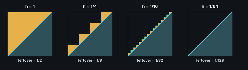
  <p>Let’s watch this happen up close. Instead of the whole staircase, zoom in on just one unit of it — the square from $x=0$ to $x=1$ — and keep refining the steps inside that same little window.</p>

  <figure class="math-figure">
  <img src="/assets/math/staircase-to-integral/zoom-sequence.svg" alt="Four panels zooming into the same unit square of the diagonal line, with step sizes one, one quarter, one sixteenth, and one sixty-fourth, showing the amber leftover thinning toward the line" />
  <figcaption>Same square, same line, four times finer each panel. The amber sliver never disappears — it just gets thinner than we can see.</figcaption>
</figure>

  <p>By the last panel, the staircase looks like a straight line. It isn’t one. Zoom the image itself in far enough on that last panel and you’d still find flat treads and square corners — 64 of them, packed into one unit. No amount of shrinking $h$ ever turns a staircase into an actual, corner-free line. It’s always built from flat steps and right angles, at every size.</p>

  <p>So here’s a precise way to say what <em>is</em> true: the staircase itself never becomes smooth. What shrinks to nothing is the <strong>gap</strong> between the staircase and the line — the amber sliver. And once that gap is gone completely, in the limit, what’s left standing is smooth — not because the staircase gradually earned smoothness, step by step, but because smoothness was a property of the line all along, and the last trace of the staircase’s roughness has been squeezed out from around it.</p>

  <p>It’s a bit like a photo made of large, visible pixels. Refine the resolution, and the pixels don’t personally get rounder or softer — they just get smaller, and smaller, until you can no longer tell they’re there. The photograph you’re approximating was smooth the entire time. The blockiness was never a rival to that smoothness. It was just the resolution you happened to be looking at it with.</p>

  <h2 id="whats-left-when-the-grain-is-gone">What’s left when the grain is gone</h2>

  <p>Let’s name what we’ve actually been computing, because the notation is about to change and it should change for a reason we can see.</p>

  <p>Every bar’s area is height times width: $k \cdot h$. Adding up all of those bar areas is a sum:</p>

\[\text{staircase area} = \sum_{k=1}^{n/h} (kh)\cdot h\]

  <p>A sum of thin rectangle areas like this, approximating the area under a line, has a name: a <strong>Riemann sum</strong>. It’s the exact thing we’ve been computing this whole time — we just didn’t have the word for it yet. $T(n)$ itself is a Riemann sum, the special case where $h=1$.</p>

  <p>We already know what this particular sum equals, because we found it by hand with the sliver picture:</p>

\[\text{staircase area} = \dfrac{n^2}{2} + \dfrac{nh}{2}\]

  <p>Now send $h$ toward 0. Nothing about the sum stops being a sum — it just ends up with more and more terms, each one thinner than the last. Take the limit of both sides:</p>

\[\lim_{h \to 0} \left( \dfrac{n^2}{2} + \dfrac{nh}{2} \right) = \dfrac{n^2}{2}\]

  <p>since we already showed $\dfrac{nh}{2} \to 0$. That limiting value — the one left standing once the grain is gone — has its own name too: the <strong>definite integral</strong> of $f(x) = x$, from 0 to $n$:</p>

\[\int_0^n x\,dx = \dfrac{n^2}{2}\]

  <p>The notation isn’t a coincidence. $\sum$ is the Greek letter sigma, for <em>sum</em>. $\int$ is a stretched-out $S$ — Leibniz’s own shorthand for <em>summa</em>, Latin for <em>sum</em>. Both symbols mean the same word. The only difference is what’s being summed: $\sum$ adds up finitely many rectangles of a fixed width $h$; $\int$ is what’s left in the limit, once that width has shrunk to 0. That’s exactly what “$dx$” means, too — it isn’t a new, mysterious infinitesimal object. It’s just the name calculus gives to $h$, once $h$ has been sent to its limit. Same quantity, different alphabet.</p>

  <p>So summation and integration were never two separate operations that happen to look alike. $\int$ <em>is</em> $\sum$, at the exact moment its rectangles become infinitely thin. Every triangular number we’ve ever computed was a Riemann sum — one with a step size fixed at exactly 1, instead of a step size carried all the way to the limit.</p>

  <p>Let’s slow down and look at two concrete examples, side by side, so this isn’t just a claim — we can watch it happen with real numbers.</p>

  <p><strong>First, $n=5$ — the case we’ve been picturing the whole time.</strong> The sum is one we already know by heart:</p>

\[\sum_{k=1}^{5} k = 1+2+3+4+5 = 15\]

  <p>And we’ve already found the integral, too, even though we didn’t call it that yet. Back when we split $T(5)$ into its two pieces, the $12.5$ we found <em>was</em> this integral all along:</p>

\[\int_0^5 x\,dx = \dfrac{5^2}{2} = 12.5\]

  <p>Subtract the integral from the sum:</p>

\[15 - 12.5 = 2.5\]

  <p>That $2.5$ is exactly $\dfrac{n}{2}$ for $n=5$ — the same leftover we’ve been tracking this entire post.</p>

  <p><strong>Now let’s check a different $n$, so we’re sure this wasn’t a coincidence.</strong> Take $n=10$. The sum:</p>

\[\sum_{k=1}^{10} k = 1+2+\cdots+10 = 55\]

  <p>The integral:</p>

\[\int_0^{10} x\,dx = \dfrac{10^2}{2} = 50\]

  <p>Subtract again:</p>

\[55 - 50 = 5\]

  <p>And $5$ is exactly $\dfrac{n}{2}$ for $n=10$. Different $n$, same relationship, right on schedule.</p>

  <p>Both times, the sum comes out a little bigger than the integral — by exactly $\dfrac{n}{2}$, never more, never less. The sum was never wrong. It’s the integral, plus one small and completely predictable extra piece, owed entirely to the fact that we counted in whole steps of $h=1$ instead of sweeping continuously.</p>

  <p>And now we can finally answer the question from earlier properly. <strong>Is the “$1$” in $\dfrac{n(n+1)}{2}$ there because the counting numbers are one apart?</strong> Yes — and now we know exactly how much of the answer that fact is responsible for. It contributes precisely $\dfrac{n}{2}$, and that whole term is the fossil of a step size of 1. Shrink the step, and the fossil shrinks with it, right on schedule, until nothing is left of it at all.</p>

  <h2 id="zero-was-never-a-destination">Zero was never a destination</h2>

  <p>It’s tempting to describe all this as “shrinking $h$ until it becomes infinitesimal” — some final, smallest possible step, just barely above zero.</p>

  <p>But there’s no such thing to land on. However small a step you pick, half of it is smaller still, and just as valid a step. There is no smallest positive number waiting at the bottom of that halving process.</p>

  <p>So what is actually being approached? Zero itself. And <a href="/blog/2026/07/19/the-deep-meaning-of-zero/">zero, we already established</a>, isn’t a quantity at all. It’s the additive identity — the point on the line with no parts left to subdivide.</p>

  <p>That’s exactly why it makes a safe target for this kind of shrinking. $h$ never has to arrive at some smallest surviving crumb of size, because it was never heading toward a quantity in the first place. It’s heading toward the one point that was never a quantity to begin with. The grain doesn’t bottom out — it just keeps finding room to get closer to a target with no size for it to bump into.</p>

  <h2 id="the-tolerance-game">The tolerance game</h2>

  <p>So mathematicians don’t ask “how small can $h$ get?” They ask a sharper question instead: <strong>can the leftover be forced below any tolerance you name, no matter how demanding?</strong></p>

  <p>Name a tolerance — call it $\varepsilon$. It can be as stingy as you like: a thousandth, a trillionth, anything positive. We need $\dfrac{nh}{2}$ to come in under it. Solve for $h$:</p>

\[\dfrac{nh}{2} &lt; \varepsilon \quad\Longleftrightarrow\quad h &lt; \dfrac{2\varepsilon}{n}\]

  <p>For any $\varepsilon &gt; 0$, choosing $h$ smaller than $\dfrac{2\varepsilon}{n}$ guarantees the leftover is smaller than $\varepsilon$. Whatever tolerance gets demanded, a step size exists that satisfies it.</p>

  <p>That, in full, is the epsilon-delta idea. Not a smallest number — a guarantee that closeness can be forced past any bar you set, on demand, forever. It replaces “there exists an infinitesimal” with something needing no controversial number at all: “for every tolerance, a response exists.” The bars in our figures were an $\varepsilon$–$\delta$ argument, drawn in color before it was ever written in symbols.</p>

  <h2 id="the-slide-was-always-there">The slide was always there</h2>

  <p>We started by asking what happens when a staircase shrinks down to nothing. The honest answer: the staircase was never the fundamental object. The slide was.</p>

  <p>The smooth line $y=x$ and its triangular area $\dfrac{n^2}{2}$ were there from the start. The staircase was just a particular, coarse way of measuring that same area — one unit-wide sliver of overcounting at a time. Discreteness wasn’t a rival to continuity. It was a grain laid on top of it, precise enough to name exactly ($\dfrac{nh}{2}$), and finable down to nothing.</p>

  <p>It’s the same reason a square’s growth and a triangle’s growth turn out to be relatives, not coincidences: $n^2$ is the sum of the first $n$ odd numbers, and $T(n-1) + T(n) = n^2$ splits that same square straight down its diagonal into two staircases. Every one of these formulas is a continuous curve, caught mid-pixelation, still recognizably itself underneath the grain.</p>

  <p>The two triangles that made a rectangle, back at the start of all this, and the triangle under a line, at the end of it, are the same shape, doing the same job, at two different resolutions.</p>

</div>]]></content><author><name>Joel Holder</name></author><category term="math" /><category term="calculus" /><category term="limits" /><category term="triangular numbers" /><category term="first principles" /><category term="integration" /><summary type="html"><![CDATA[]]></summary><media:thumbnail xmlns:media="http://search.yahoo.com/mrss/" url="https://joelholder.com/assets/hero/the-staircase-and-the-slide.png" /><media:content medium="image" url="https://joelholder.com/assets/hero/the-staircase-and-the-slide.png" xmlns:media="http://search.yahoo.com/mrss/" /></entry><entry><title type="html">Looking Deeper at the Meaning of Zero</title><link href="https://joelholder.com/blog/2026/07/19/the-deep-meaning-of-zero/" rel="alternate" type="text/html" title="Looking Deeper at the Meaning of Zero" /><published>2026-07-19T19:00:00+00:00</published><updated>2026-07-19T19:00:00+00:00</updated><id>https://joelholder.com/blog/2026/07/19/the-deep-meaning-of-zero</id><content type="html" xml:base="https://joelholder.com/blog/2026/07/19/the-deep-meaning-of-zero/"><![CDATA[<style>
.zero-post .katex-display,
.zero-post .katex-display > .katex {
  text-align: left !important;
}
.zero-post .katex-display > .katex {
  font-size: 1.4em !important;
}
.zero-post svg { margin-left: 0 !important; margin-right: auto !important; }
</style>

<div class="zero-post">

  <p>Every number is defined by where it sits in the continuum relative to one fixed point. That point is zero.  It can be thought of the beginning of addition.</p>

  <p>Zero is the <em>Unit</em> of addition, giving us back the identity of a thing when we add zero to that thing.</p>

  <p>It turns out to have two descriptions that are really the same fact:</p>

  <p>  <strong>Algebra</strong> - <strong>the operation that changes nothing</strong></p>

  <p>  <strong>Geometry</strong> - <strong>that which has no parts</strong></p>

  <p>Zero cannot be subdivided. It cannot be scaled. It cannot be denominated.</p>

  <h2 id="the-additive-identity-the-operation-that-changes-nothing">The additive identity: the operation that changes nothing</h2>

\[a + 0 = a\]

  <p>Adding $0$ never changes $a$. That’s the whole definition: $0$ isn’t a quantity. Adding it to a number does <strong>nothing</strong>. Every other number does something when added to $a$.</p>

  <h2 id="zero--euclids-point-the-geometric-construct-of-nothingness">Zero = Euclid’s point: the geometric construct of nothingness</h2>

  <p><em>A point is that which has no part</em> — no length, nothing to divide.</p>

  <div style="padding:1rem 0;">
<svg viewBox="0 0 640 200" style="width:100%;max-width:640px;display:block;margin:0;">
  <line x1="220" y1="45" x2="320" y2="45" stroke="#5fd38d" stroke-width="4" />
  <line x1="320" y1="45" x2="420" y2="45" stroke="#64c7d8" stroke-width="4" />
  <line x1="320" y1="32" x2="320" y2="58" stroke="#0e1418" stroke-width="2" />
  <text x="320" y="78" fill="#9caab4" font-size="16" text-anchor="middle">a quantity — cut here, two parts</text>

  <circle cx="320" cy="130" r="6" fill="#f2f5f3" />
  <text x="320" y="164" fill="#f2f5f3" font-size="16" text-anchor="middle" font-weight="700">
      zero — no parts to cut
  </text>
</svg>
</div>
  <p>A segment can always be cut somewhere. Zero has no dimension to put a cut in.</p>

  <h2 id="the-operational-symmetry-of-a-and--a">The operational symmetry of $+a$ and $-a$</h2>

  <p>Think of $+a$ not as a number but as a <em>move</em>: take whatever you have, apply $+a$ to it. It has a mirror move, $-a$, defined by one property:</p>

\[a + (-a) = 0\]

  <p>Apply $+a$, then $-a$. Or apply $-a$, then $+a$. Either order, the two moves compose into the do-nothing move. Neither one is “more basic” than the other — that’s the symmetry. Each is exactly what the other one requires to return you to identity, and that requirement is the <em>entire</em> definition of an inverse. Nothing physical about it; it’s a statement about how two operations compose.</p>

  <h2 id="does-the-symmetry-survive-combining-numbers">Does the symmetry survive combining numbers?</h2>

  <p>Apply $+a$, then $+b$. Then $-a$, then $-b$. Does the whole chain still compose to the identity?</p>

  <svg viewBox="0 0 640 190" style="width:100%;max-width:640px;display:block;margin:1.5rem 0;">
  <defs>
    <marker id="pf-g" markerWidth="9" markerHeight="9" refX="7" refY="4.5" orient="auto"><path d="M0,0 L9,4.5 L0,9 Z" fill="#5fd38d" /></marker>
    <marker id="pf-c" markerWidth="9" markerHeight="9" refX="7" refY="4.5" orient="auto"><path d="M0,0 L9,4.5 L0,9 Z" fill="#64c7d8" /></marker>
    <marker id="pf-a" markerWidth="9" markerHeight="9" refX="7" refY="4.5" orient="auto"><path d="M0,0 L9,4.5 L0,9 Z" fill="#f2b84b" /></marker>
    <marker id="pf-r" markerWidth="9" markerHeight="9" refX="7" refY="4.5" orient="auto"><path d="M0,0 L9,4.5 L0,9 Z" fill="#f38ba8" /></marker>
  </defs>
  <line x1="20" y1="95" x2="620" y2="95" stroke="#3a4650" stroke-width="1.5" />
  <line x1="320" y1="85" x2="320" y2="105" stroke="#3a4650" stroke-width="1.5" />
  <text x="320" y="128" fill="#9caab4" font-size="16" text-anchor="middle">identity</text>

  <line x1="323" y1="72" x2="418" y2="72" stroke="#5fd38d" stroke-width="3" marker-end="url(#pf-g)" />
  <text x="370" y="57" fill="#5fd38d" font-size="17" text-anchor="middle">+a</text>

  <line x1="420" y1="40" x2="515" y2="40" stroke="#64c7d8" stroke-width="3" marker-end="url(#pf-c)" />
  <text x="467" y="25" fill="#64c7d8" font-size="17" text-anchor="middle">+b</text>

  <line x1="518" y1="118" x2="423" y2="118" stroke="#f2b84b" stroke-width="3" marker-end="url(#pf-a)" />
  <text x="470" y="140" fill="#f2b84b" font-size="17" text-anchor="middle">−a</text>

  <line x1="420" y1="150" x2="325" y2="150" stroke="#f38ba8" stroke-width="3" marker-end="url(#pf-r)" />
  <text x="372" y="172" fill="#f38ba8" font-size="17" text-anchor="middle">−b</text>

  <circle cx="320" cy="95" r="5" fill="#f2f5f3" />
  <circle cx="518" cy="95" r="4" fill="#5a6875" />
</svg>

  <p>Yes — it is necessarily so, by two rules you already know and trust:</p>

  <ol>
    <li>reorder freely (<strong>commutativity</strong>)</li>
    <li>regroup freely (<strong>associativity</strong>)</li>
  </ol>

\[\begin{aligned}
(a+b) + (-a+-b) &amp;= a + b + (-a) + (-b) &amp;&amp;\text{(associativity)} \\
&amp;= a + (-a) + b + (-b) &amp;&amp;\text{(commutativity)} \\
&amp;= \big(a + (-a)\big) + \big(b + (-b)\big) &amp;&amp;\text{(associativity)} \\
&amp;= 0 + 0 = 0
\end{aligned}\]

  <p>$-a$ composing with $a$ to give $0$ isn’t a discovered fact about the world.</p>

  <p>It’s what the words mean: an inverse is, by definition, the move that composes with the original move to produce the identity.</p>

</div>]]></content><author><name>Joel Holder</name></author><category term="math" /><category term="first principles" /><category term="zero" /><category term="proofs" /><category term="number line" /><category term="inverses" /><summary type="html"><![CDATA[]]></summary></entry><entry><title type="html">Remote C++ Development Over SSH: No GUI Required</title><link href="https://joelholder.com/blog/2026/07/17/remote-cpp-development-with-emacs-over-ssh/" rel="alternate" type="text/html" title="Remote C++ Development Over SSH: No GUI Required" /><published>2026-07-17T23:30:00+00:00</published><updated>2026-07-17T23:30:00+00:00</updated><id>https://joelholder.com/blog/2026/07/17/remote-cpp-development-with-emacs-over-ssh</id><content type="html" xml:base="https://joelholder.com/blog/2026/07/17/remote-cpp-development-with-emacs-over-ssh/"><![CDATA[<div style="position:relative;padding-bottom:56.25%;height:0;overflow:hidden;max-width:100%;margin:1rem 0;">
  <iframe src="https://www.youtube-nocookie.com/embed/HLhSy1cB6Lw" title="YouTube video player" style="position:absolute;top:0;left:0;width:100%;height:100%;border:0;" allow="accelerometer; autoplay; clipboard-write; encrypted-media; gyroscope; picture-in-picture; web-share" referrerpolicy="strict-origin-when-cross-origin" allowfullscreen="">
  </iframe>
</div>

<p><em>A full IDE running inside nothing but an SSH session. No GUI. No lag. No lock-in.</em></p>

<p><strong>Config, MIT licensed:</strong> <a href="https://github.com/jclosure/vscode-flavored-emacs-2026">github.com/jclosure/vscode-flavored-emacs-2026</a></p>

<h2 id="the-case-for-terminal-only-development">The case for terminal-only development</h2>

<p>Here’s the thing nobody tells you: the IDE you’ve been dragging across the network — the file tree, the extension marketplace, the remote-desktop handshake — none of it was ever the point. The point was always completion, navigation, refactoring, and debugging. Everything else is just weight.</p>

<p>Strip it down to a terminal, an SSH connection, and Emacs, and you get all four, running natively on the machine that actually has your code, your compiler, your build. Zero latency between you and it, because there’s no picture being pushed across the wire — just keystrokes and text, the two things a network connection has always been good at.</p>

<p>This isn’t old tech because it’s outdated. It’s old tech because it’s proven, and it turns out the fastest, most portable interface between a human and a remote machine was never a rendered window. It was text. This just points that idea at a modern problem.</p>

<h2 id="simple">Simple</h2>

<p>One program. One set of keybindings that works the same whether you’re on your laptop or SSH’d three hops deep into a box you don’t even own. No juggling a local editor, a remote-desktop client, and a file-sync tool at the same time. You open a terminal, type <code class="language-plaintext highlighter-rouge">ssh</code>, and you’re already inside your actual development environment — not a shadow of it, waiting to sync.</p>

<h2 id="powerful">Powerful</h2>

<p>This isn’t a stripped-down, “good enough for a text editor” version of a real IDE. Autocomplete knows your types. Errors surface as you type them. Jump-to-definition takes you into the real standard library source, not a stub. Rename a function and every call site updates, project-wide. Set a breakpoint, step through it, inspect a variable live — all inside the same terminal window you started in.</p>

<p>You could be on a train with spotty wifi, or SSH’d into a machine on the other side of the planet, and it behaves identically either way. That’s not a compromise you’re making. That’s the actual advantage.</p>

<h2 id="you-dont-need-to-already-be-an-emacs-wizard">You don’t need to already be an Emacs wizard</h2>

<p>This isn’t a “prove yourself first” tool. It’s a config — pre-built, documented, and free to just clone and point at your own project. The IDE part works immediately. Whatever else you want to do with the forty years of Emacs sitting underneath it is entirely optional, and entirely up to you, whenever you’re ready for it.</p>

<p><strong>Try it:</strong> <a href="https://github.com/jclosure/vscode-flavored-emacs-2026">github.com/jclosure/vscode-flavored-emacs-2026</a> — MIT licensed, no strings attached.</p>]]></content><author><name>Joel Holder</name></author><category term="emacs" /><category term="tools" /><category term="emacs" /><category term="ssh" /><category term="c++" /><category term="remote development" /><category term="terminal" /><summary type="html"><![CDATA[]]></summary></entry><entry><title type="html">Gauss, Pascal, and Triangular Numbers</title><link href="https://joelholder.com/blog/2026/07/13/gauss-pascal-and-triangular-numbers/" rel="alternate" type="text/html" title="Gauss, Pascal, and Triangular Numbers" /><published>2026-07-13T04:06:00+00:00</published><updated>2026-07-13T04:06:00+00:00</updated><id>https://joelholder.com/blog/2026/07/13/gauss-pascal-and-triangular-numbers</id><content type="html" xml:base="https://joelholder.com/blog/2026/07/13/gauss-pascal-and-triangular-numbers/"><![CDATA[<p>Before we talk about formulas, start with a picture.</p>

<p>If we stack blocks in rows of 1, then 2, then 3, and keep going, we get a triangle. Let $n$ be the number we count up to. In the picture below, $n = 5$, so the triangle has 5 rows.</p>

\[1 + 2 + 3 + 4 + 5\]

<p>The running totals show how the count grows. The dot picture shows the same thing as rows of blocks:</p>

<div class="running-dot-grid">
  <div class="running-total-list">
    <p><strong>Running totals</strong></p>

    <p class="step-formula">\(1 = 1\)</p>
    <p class="step-formula">\(1 + 2 = 3\)</p>
    <p class="step-formula">\(1 + 2 + 3 = 6\)</p>
    <p class="step-formula">\(1 + 2 + 3 + 4 = 10\)</p>
    <p class="step-formula">\(1 + 2 + 3 + 4 + 5 = 15\)</p>
    <div class="running-note">15 = running total</div>
  </div>

  <div class="dot-triangle">
  <strong>Dot picture</strong>
  <div>&bull;</div>
  <div>&bull; &bull;</div>
  <div>&bull; &bull; &bull;</div>
  <div>&bull; &bull; &bull; &bull;</div>
  <div>&bull; &bull; &bull; &bull; &bull;</div>
  <div class="dot-note">15 dots = area \(T\)</div>
</div>
</div>

<p>Let $T$ be the number of blocks in that triangle. Our goal is to find $T$ without counting every block one at a time.</p>

<p>Now make a copy of the same triangle, flip it, and put the two pieces together. The two triangles form a rectangle.</p>

<figure class="math-figure">
  <img src="/assets/math/gauss-pascal-triangular/triangle-rectangle-proof.svg" alt="A triangular stack copied and flipped to make a rectangle" />
  <figcaption>A triangular stack is half of a rectangle.</figcaption>
</figure>

<p>Each small block has area 1 block-unit. So counting blocks is the same as computing area in block-units.</p>

<p>For the example with $n = 5$, the calculation is:</p>

<div class="proof-sequence">
  <div class="proof-step">
    <p><strong>Rectangle area</strong></p>

    <p class="step-formula">\(5 \cdot 6 = 30\)</p>
  </div>

  <div class="proof-step">
    <p><strong>Half the rectangle</strong></p>

    <p class="step-formula">\(T = 30 / 2 = 15\)</p>
  </div>
</div>

<p>The picture suggests the general rule. If the triangle has $n$ rows, the doubled rectangle has $n$ rows and $n + 1$ columns. Its area is $n(n + 1)$ block-units. The triangle is half the rectangle, so:</p>

\[T = \frac{n(n + 1)}{2}\]

<p>But a picture is not quite a proof. It gives us the idea. Now we want to prove the idea with algebra.</p>

<p>That is where Gauss’s trick comes in.</p>

<p>Suppose we want to add the numbers from 1 to 100. Here $n = 100$, and $T$ is the total we are trying to find:</p>

\[1 + 2 + 3 + \dots + 98 + 99 + 100\]

<p>Gauss’s trick is to write the same total twice: once forward, and once backward.</p>

\[\begin{array}{rrrrrrrr}
T = &amp; 1   &amp; + 2  &amp; + 3  &amp; + \dots &amp; + 98 &amp; + 99 &amp; + 100 \\
T = &amp; 100 &amp; + 99 &amp; + 98 &amp; + \dots &amp; + 3  &amp; + 2  &amp; + 1
\end{array}\]

<p>Now add the two rows together. Associativity lets us group the sum by columns: first with first, second with second, third with third, and so on.</p>

<div class="proof-sequence">
  <div class="proof-step">
    <p><strong>Pair the columns</strong></p>

    <p class="step-formula">\(2T = (1 + 100) + (2 + 99) + \dots + (100 + 1)\)</p>
  </div>

  <div class="proof-step">
    <p><strong>Notice the repeated sum</strong></p>

    <p class="step-formula">\(2T = 101 + 101 + \dots + 101\)</p>
  </div>

  <div class="proof-step">
    <p><strong>Count the pairs</strong></p>

    <p class="step-formula">\(2T = 100 \cdot 101\)</p>
  </div>
</div>

<p>Each column-pair adds to 101, and there are 100 pairs. This is the same idea as the block picture: 100 rows, 101 columns, and twice the triangle.</p>

<p>Since $2T$ is twice the original total, divide by 2:</p>

\[T = \frac{100 \cdot 101}{2} = 5050\]

<p>The important step is not the number 5050. The important step is the pairing.</p>

<p>The same proof works for any $n$. Write the total forward and backward:</p>

\[\begin{array}{rrrrrr}
T(n) = &amp; 1 &amp; + 2 &amp; + 3 &amp; + \dots &amp; + n \\
T(n) = &amp; n &amp; + (n - 1) &amp; + (n - 2) &amp; + \dots &amp; + 1
\end{array}\]

<p>Then use associativity to group the columns into pairs:</p>

<div class="proof-sequence">
  <div class="proof-step">
    <p><strong>Pair the columns</strong></p>

    <p class="step-formula">\(2T(n) = (1 + n) + (2 + (n - 1)) + \dots + (n + 1)\)</p>
  </div>

  <div class="proof-step">
    <p><strong>Notice the repeated sum</strong></p>

    <p class="step-formula">\(2T(n) = (n + 1) + (n + 1) + \dots + (n + 1)\)</p>
  </div>

  <div class="proof-step">
    <p><strong>Count the pairs</strong></p>

    <p class="step-formula">\(2T(n) = n(n + 1)\)</p>
  </div>
</div>

<p>Every pair adds to $n + 1$, and there are $n$ pairs. Divide by 2 and we get:</p>

\[T(n) = \frac{n(n + 1)}{2}\]

<p>That proves the formula behind the rectangle picture. The algebra and the geometry are saying the same thing.</p>

<p>Now we can connect this to Pascal’s triangle.</p>

<p>Pascal’s triangle is built by addition. Every inside number is the sum of the two numbers above it:</p>

\[\begin{array}{ccccccccccc}
&amp;&amp;&amp;&amp;&amp;1&amp;&amp;&amp;&amp;&amp;\\
&amp;&amp;&amp;&amp;1&amp;&amp;1&amp;&amp;&amp;&amp;\\
&amp;&amp;&amp;1&amp;&amp;2&amp;&amp;1&amp;&amp;&amp;\\
&amp;&amp;1&amp;&amp;3&amp;&amp;3&amp;&amp;1&amp;&amp;\\
&amp;1&amp;&amp;4&amp;&amp;6&amp;&amp;4&amp;&amp;1&amp;\\
1&amp;&amp;5&amp;&amp;10&amp;&amp;10&amp;&amp;5&amp;&amp;1
\end{array}\]

<p>For example, the 6 is made from the two 3s above it:</p>

\[\begin{array}{ccccc}
&amp; 3 &amp;&amp; 3 &amp;\\
&amp; \searrow &amp;&amp; \swarrow &amp;\\
&amp;&amp; 3 + 3 = 6 &amp;&amp;
\end{array}\]

<p>The edge numbers stay 1. The inside numbers are where the adding happens.</p>

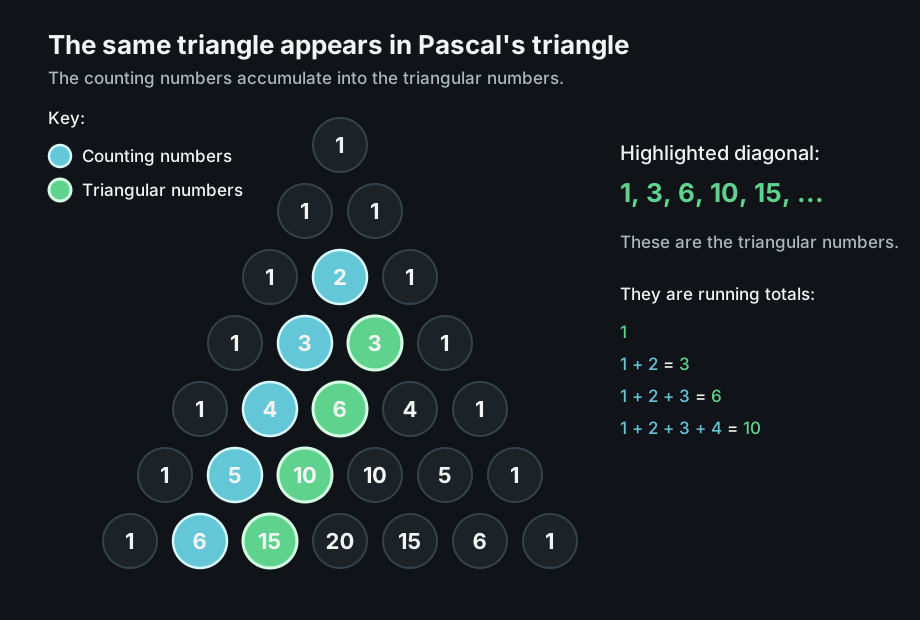
<p>The counting numbers appear along one diagonal:</p>

\[1,\ 2,\ 3,\ 4,\ 5,\ \dots\]

<p>The next diagonal keeps a running total of those counting numbers:</p>

\[1,\quad 1 + 2,\quad 1 + 2 + 3,\quad 1 + 2 + 3 + 4,\quad \dots\]

<p>That gives:</p>

\[1,\ 3,\ 6,\ 10,\ 15,\ \dots\]

<p>Those are the same triangular totals we just proved.</p>
<figure class="math-figure">
  <img src="/assets/math/gauss-pascal-triangular/pascal-triangle-diagonal.svg" alt="The triangular numbers highlighted in Pascal's triangle" />
  <figcaption>The triangular numbers appear as a diagonal in Pascal's triangle.</figcaption>
</figure>

<p>So the same idea appears in three forms:</p>

\[1 + 2 + 3 + 4 + 5 + 6 + \dots + n = \frac{n(n + 1)}{2}\]

<p>The block picture shows why the triangle is half of a rectangle. Gauss’s pairing turns that picture into a proof. Pascal’s triangle shows the same repeated addition hiding inside a larger pattern.</p>]]></content><author><name>Joel Holder</name></author><category term="math" /><category term="proofs" /><category term="pascal&apos;s triangle" /><category term="triangular numbers" /><category term="gauss" /><category term="first principles" /><summary type="html"><![CDATA[Before we talk about formulas, start with a picture.]]></summary></entry><entry><title type="html">A Tiny Proof From First Principles</title><link href="https://joelholder.com/blog/2026/07/11/a-tiny-proof-from-first-principles/" rel="alternate" type="text/html" title="A Tiny Proof From First Principles" /><published>2026-07-11T05:43:00+00:00</published><updated>2026-07-11T05:43:00+00:00</updated><id>https://joelholder.com/blog/2026/07/11/a-tiny-proof-from-first-principles</id><content type="html" xml:base="https://joelholder.com/blog/2026/07/11/a-tiny-proof-from-first-principles/"><![CDATA[<p>One of the pleasures of pure math is how far you can travel with very small tools.</p>

<p>Before the symbols become intimidating, before the machinery becomes elaborate, there are laws so simple they almost disappear into common sense. Two of the most important are associativity and commutativity.</p>

<p>Commutativity says that order does not matter for addition:</p>

\[x + y = y + x\]

<p>Associativity says that grouping does not matter for addition:</p>

\[(x + y) + z = x + (y + z)\]

<p>These are tiny statements. But they give us permission to reorganize a sum without changing its value. That permission is powerful.</p>

<p>Consider this identity:</p>

\[(a + b) + (c + d) = (a + d) + (b + c)\]

<p>At first glance, the right side looks like a rearrangement by instinct. But a proof should not rely on instinct. It should show exactly which moves are allowed.</p>

<p>Starting on the left:</p>

\[\begin{aligned}
(a + b) + (c + d)
&amp;= a + \bigl(b + (c + d)\bigr) &amp;&amp; \text{associativity} \\
&amp;= a + \bigl((b + c) + d\bigr) &amp;&amp; \text{associativity} \\
&amp;= a + \bigl(d + (b + c)\bigr) &amp;&amp; \text{commutativity} \\
&amp;= (a + d) + (b + c) &amp;&amp; \text{associativity}
\end{aligned}\]

<p>That is the whole proof.</p>

<p>The lovely thing is that nothing fancy happened. We did not calculate. We did not expand into a more complicated system. We simply used two first principles to move parentheses and reorder terms.</p>

<p>This is what makes proof feel different from arithmetic. Arithmetic often asks, “What is the answer?” Proof asks, “What transformations are legitimate?” Once the rules are clear, the path becomes visible.</p>

<p>In this small identity, associativity lets us change the shape of the expression. Commutativity lets us change the order. Together, they turn a rigid-looking formula into something flexible:</p>

\[(a + b) + (c + d)
\quad \longrightarrow \quad
(a + d) + (b + c)\]

<p>That flexibility is not a trick. It is structure. And much of mathematics is the art of noticing which structures give us freedom, then learning how to move beautifully inside them.</p>]]></content><author><name>Joel Holder</name></author><category term="math" /><category term="pure math" /><category term="proofs" /><category term="first principles" /><category term="algebra" /><summary type="html"><![CDATA[One of the pleasures of pure math is how far you can travel with very small tools.]]></summary></entry><entry><title type="html">Automata Arcade Is Becoming an Instrument</title><link href="https://joelholder.com/blog/2026/05/20/automata-arcade-is-becoming-an-instrument/" rel="alternate" type="text/html" title="Automata Arcade Is Becoming an Instrument" /><published>2026-05-20T06:38:03+00:00</published><updated>2026-05-20T06:38:03+00:00</updated><id>https://joelholder.com/blog/2026/05/20/automata-arcade-is-becoming-an-instrument</id><content type="html" xml:base="https://joelholder.com/blog/2026/05/20/automata-arcade-is-becoming-an-instrument/"><![CDATA[<p><em>Automata Arcade now has selection transforms, lenses, zones, and manifold-mapped regions. The project is shifting from a cellular automata sandbox into a small workbench for building, inspecting, and reusing emergent systems.</em></p>
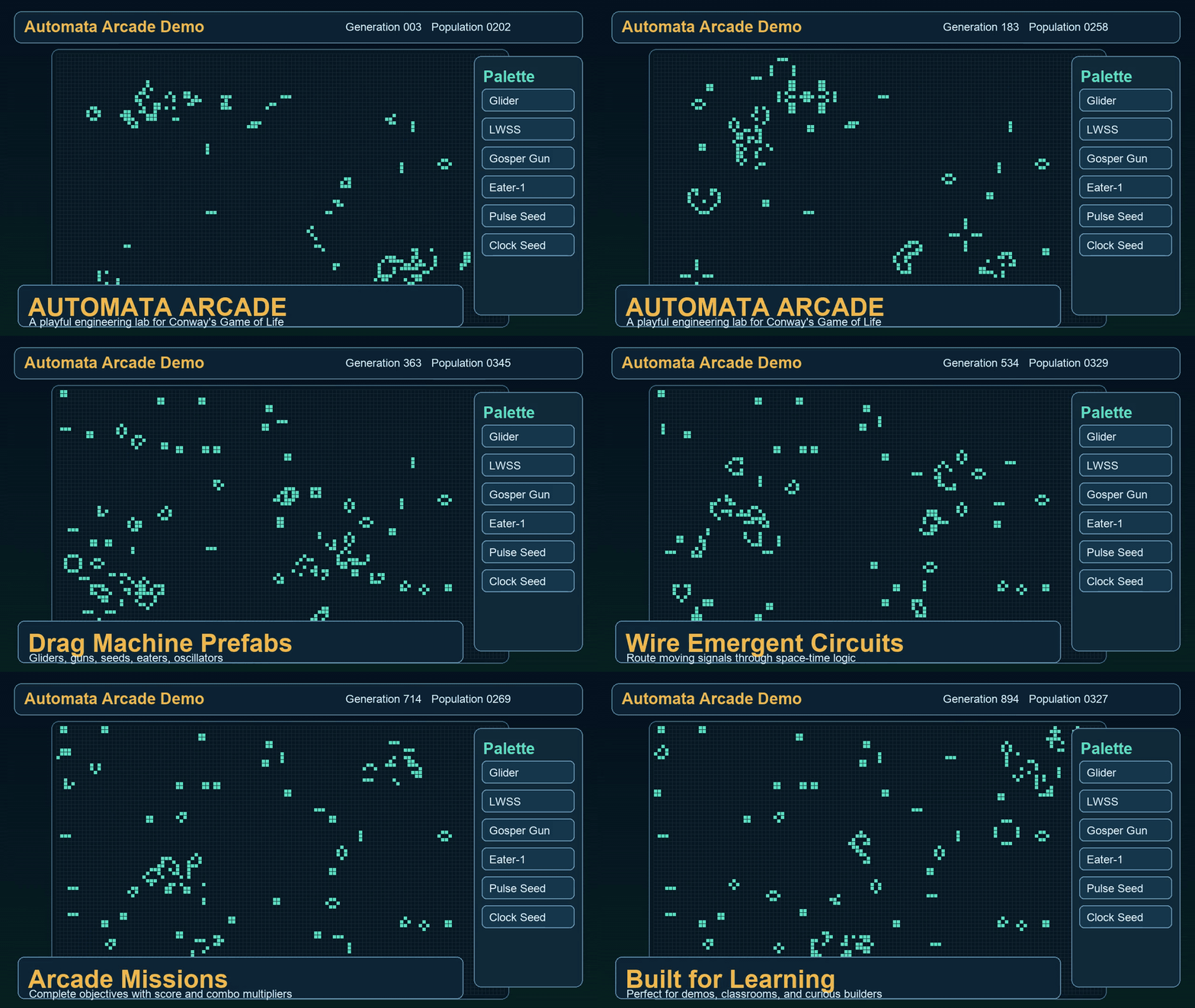
<p>Automata Arcade started as a simple cellular automata canvas: paint cells, run the simulation, watch the pattern evolve.</p>
<p>That loop is still there, but the tool now supports the operations needed for serious iteration: select, transform, inspect, isolate, map, and reuse.</p>
<p>Try it here: <a href="https://automata-arcade.vercel.app">Automata Arcade live demo</a> · <a href="https://github.com/jclosure/automata-arcade">GitHub repository</a></p>
<h2>The board is editable</h2>
<p>Selection mode turns a region of cells into an object you can operate on. You can draw a rectangular selection, translate it, rotate it 90 degrees, flip it, copy it, cut it, paste it, and save the result as a prefab.</p>
<p>For cellular automata, that matters. A glider stream, oscillator, eater, failed collision, or partial circuit is no longer just transient state on the board. It becomes material.</p>
<p>The workflow changes from redrawing patterns by hand to editing mechanisms directly:</p>
<ol>
<li>observe a behavior</li>
<li>select the active region</li>
<li>transform or duplicate it</li>
<li>test the new geometry</li>
<li>save the useful result</li>
</ol>
<p>That is the basic interaction model for an automata workbench.</p>
<h2>Lenses keep local behavior readable</h2>
<p>Lenses are circular magnifiers placed directly on the canvas. They enlarge a local region without zooming the whole board.</p>
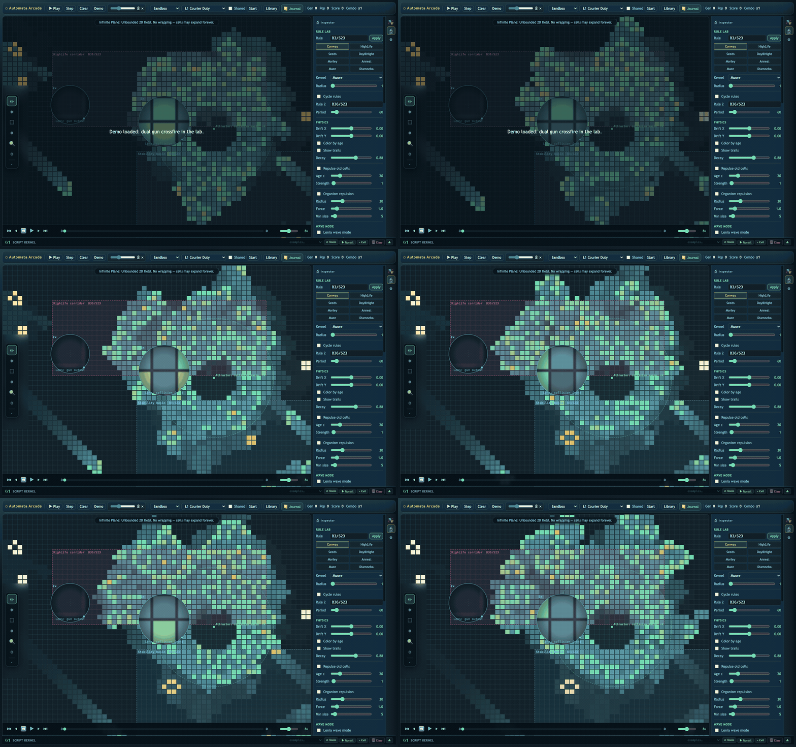
<figure class="wp-block-image size-large"><img data-recalc-dims="1" loading="lazy" decoding="async" width="960" height="600" data-attachment-id="1807" data-permalink="https://joelholder.com/01-lenses-zones-fields-live-2/" data-orig-file="https://i0.wp.com/joelholder.com/wp-content/uploads/2026/05/01-lenses-zones-fields-live.gif?fit=960%2C600&amp;ssl=1" data-orig-size="960,600" data-comments-opened="1" data-image-meta="{&quot;aperture&quot;:&quot;0&quot;,&quot;credit&quot;:&quot;&quot;,&quot;camera&quot;:&quot;&quot;,&quot;caption&quot;:&quot;&quot;,&quot;created_timestamp&quot;:&quot;0&quot;,&quot;copyright&quot;:&quot;&quot;,&quot;focal_length&quot;:&quot;0&quot;,&quot;iso&quot;:&quot;0&quot;,&quot;shutter_speed&quot;:&quot;0&quot;,&quot;title&quot;:&quot;&quot;,&quot;orientation&quot;:&quot;0&quot;}" data-image-title="01-lenses-zones-fields-live" data-image-description="" data-image-caption="" data-large-file="https://i0.wp.com/joelholder.com/wp-content/uploads/2026/05/01-lenses-zones-fields-live.gif?fit=960%2C600&amp;ssl=1" src="/assets/wp/automata-arcade-is-becoming-an-instrument/01-lenses-zones-fields-live.gif" alt="A short capture of lenses and zones while the automaton evolves" class="wp-image-1807" /><figcaption>A short capture of lenses and zones while the automaton evolves</figcaption></figure>
<p>Automata are multiscale. You often need neighbor-level detail and board-level context at the same time: births, deaths, phase offsets, collision fronts, stream timing, boundaries, and population waves.</p>
<p>A normal zoom makes you choose between those views. Lenses let you keep both.</p>
<p>You can place one lens over a generator, another over a collision site, and compare cause and effect while the simulation runs.</p>
<h2>Zones make rules spatial</h2>
<p>Zones are rectangular regions with rule overrides. A cell can move from classic Life into HighLife, Seeds, Day &amp; Night, or a custom B/S rule without leaving the board.</p>
<p>That makes the plane heterogeneous. A zone can act as a reaction chamber, protected basin, hostile boundary, rule-gradient experiment, or computational component.</p>
<p>The question becomes more precise: what happens when a structure crosses from one local physics into another?</p>
<p>That is useful for design, debugging, and play. It also gives rule changes a spatial form instead of treating them as global configuration.</p>
<h2>Manifold regions make topology local</h2>
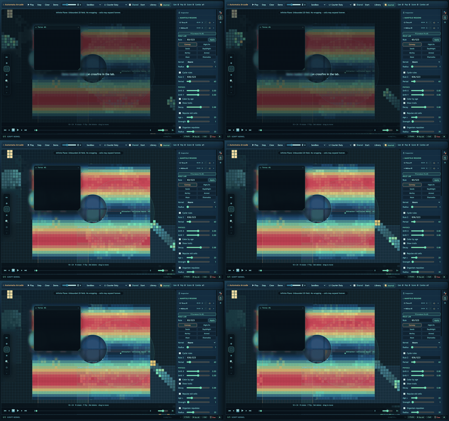
<p>Manifold Regions map a rectangular patch of the flat board onto a topology such as a sphere, torus, Möbius strip, or Klein bottle.</p>
<figure class="wp-block-image size-large"><img data-recalc-dims="1" loading="lazy" decoding="async" width="960" height="600" data-attachment-id="1809" data-permalink="https://joelholder.com/03-manifold-regions-curvature/" data-orig-file="https://i0.wp.com/joelholder.com/wp-content/uploads/2026/05/03-manifold-regions-curvature.gif?fit=960%2C600&amp;ssl=1" data-orig-size="960,600" data-comments-opened="1" data-image-meta="{&quot;aperture&quot;:&quot;0&quot;,&quot;credit&quot;:&quot;&quot;,&quot;camera&quot;:&quot;&quot;,&quot;caption&quot;:&quot;&quot;,&quot;created_timestamp&quot;:&quot;0&quot;,&quot;copyright&quot;:&quot;&quot;,&quot;focal_length&quot;:&quot;0&quot;,&quot;iso&quot;:&quot;0&quot;,&quot;shutter_speed&quot;:&quot;0&quot;,&quot;title&quot;:&quot;&quot;,&quot;orientation&quot;:&quot;0&quot;}" data-image-title="03-manifold-regions-curvature" data-image-description="" data-image-caption="" data-large-file="https://i0.wp.com/joelholder.com/wp-content/uploads/2026/05/03-manifold-regions-curvature.gif?fit=960%2C600&amp;ssl=1" src="/assets/wp/automata-arcade-is-becoming-an-instrument/03-manifold-regions-curvature.gif" alt="A short capture of automata evolving across manifold-mapped regions" class="wp-image-1809" /><figcaption>A short capture of automata evolving across manifold-mapped regions</figcaption></figure>
<p>The whole board does not need to become a torus. A local patch can have toroidal adjacency while the surrounding workspace stays flat. Another patch can contain a Möbius seam.</p>
<p>This makes topology an editable part of the system. The same rule and seed can behave differently because the neighborhood graph changed.</p>
<p>For cellular automata, the rule is not the whole machine. Initial condition, observation, tools, and geometry all matter. Manifold Regions make the geometry explicit.</p>
<h2>The IDE shape</h2>
<p>Several systems are now converging:</p>
<ul>
<li>canvas tools: paint, select, transform, stamp</li>
<li>analysis tools: period detection, population tracking, heatmaps</li>
<li>rule tools: presets, B/S editing, kernel radius, Lenia controls</li>
<li>spatial tools: zones, force fields, lenses</li>
<li>topology tools: manifold regions and curvature visualization</li>
<li>journal/script tools: documented, replayable experiments</li>
</ul>
<p>The next useful step is persistence. Experiments should capture board state, rule configuration, selected regions, camera and lens positions, script cells, manifold mappings, and replayable timelines.</p>
<p>Prefabs should also become structured objects instead of screenshots: period, bounding box, velocity, input/output lanes, required phase, compatible rules, and known failure modes.</p>
<p>After that, topology can become a programming surface. Region seams, wraps, and local adjacency changes could be used as parts of spatial circuits.</p>
<p>The longer-term direction is an interactive atlas: scenes, rules, mechanisms, manifolds, and experiments that can be inspected, forked, mutated, and republished.</p>
<p>Automata Arcade is still an arcade. The play matters. But the current direction is clear: it is becoming an instrument for composing and studying cellular automata.</p>]]></content><author><name>Joel Holder</name></author><category term="Automata Arcade" /><category term="cellular automata" /><category term="creative coding" /><category term="manifolds" /><category term="simulation" /><summary type="html"><![CDATA[Automata Arcade now has selection transforms, lenses, zones, and manifold-mapped regions. The project is shifting from a cellular automata sandbox into a small workbench for building, inspecting, and reusing emergent systems. Automata Arcade started as a simple cellular automata canvas: paint cells, run the simulation, watch the pattern evolve. That loop is still there, but the tool now supports the operations needed for serious iteration: select, transform, inspect, isolate, map, and reuse. Try it here: Automata Arcade live demo · GitHub repository The board is editable Selection mode turns a region of cells into an object you can operate on. You can draw a rectangular selection, translate it, rotate it 90 degrees, flip it, copy it, cut it, paste it, and save the result as a prefab. For cellular automata, that matters. A glider stream, oscillator, eater, failed collision, or partial circuit is no longer just transient state on the board. It becomes material. The workflow changes from redrawing patterns by hand to editing mechanisms directly: observe a behavior select the active region transform or duplicate it test the new geometry save the useful result That is the basic interaction model for an automata workbench. Lenses keep local behavior readable Lenses are circular magnifiers placed directly on the canvas. They enlarge a local region without zooming the whole board. A short capture of lenses and zones while the automaton evolves Automata are multiscale. You often need neighbor-level detail and board-level context at the same time: births, deaths, phase offsets, collision fronts, stream timing, boundaries, and population waves. A normal zoom makes you choose between those views. Lenses let you keep both. You can place one lens over a generator, another over a collision site, and compare cause and effect while the simulation runs. Zones make rules spatial Zones are rectangular regions with rule overrides. A cell can move from classic Life into HighLife, Seeds, Day &amp; Night, or a custom B/S rule without leaving the board. That makes the plane heterogeneous. A zone can act as a reaction chamber, protected basin, hostile boundary, rule-gradient experiment, or computational component. The question becomes more precise: what happens when a structure crosses from one local physics into another? That is useful for design, debugging, and play. It also gives rule changes a spatial form instead of treating them as global configuration. Manifold regions make topology local Manifold Regions map a rectangular patch of the flat board onto a topology such as a sphere, torus, Möbius strip, or Klein bottle. A short capture of automata evolving across manifold-mapped regions The whole board does not need to become a torus. A local patch can have toroidal adjacency while the surrounding workspace stays flat. Another patch can contain a Möbius seam. This makes topology an editable part of the system. The same rule and seed can behave differently because the neighborhood graph changed. For cellular automata, the rule is not the whole machine. Initial condition, observation, tools, and geometry all matter. Manifold Regions make the geometry explicit. The IDE shape Several systems are now converging: canvas tools: paint, select, transform, stamp analysis tools: period detection, population tracking, heatmaps rule tools: presets, B/S editing, kernel radius, Lenia controls spatial tools: zones, force fields, lenses topology tools: manifold regions and curvature visualization journal/script tools: documented, replayable experiments The next useful step is persistence. Experiments should capture board state, rule configuration, selected regions, camera and lens positions, script cells, manifold mappings, and replayable timelines. Prefabs should also become structured objects instead of screenshots: period, bounding box, velocity, input/output lanes, required phase, compatible rules, and known failure modes. After that, topology can become a programming surface. Region seams, wraps, and local adjacency changes could be used as parts of spatial circuits. The longer-term direction is an interactive atlas: scenes, rules, mechanisms, manifolds, and experiments that can be inspected, forked, mutated, and republished. Automata Arcade is still an arcade. The play matters. But the current direction is clear: it is becoming an instrument for composing and studying cellular automata.]]></summary></entry><entry><title type="html">Automata Arcade: Building a Playable Lab for Conway’s Game of Life</title><link href="https://joelholder.com/blog/2026/03/08/automata-arcade-building-a-playable-lab-for-conways-game-of-life/" rel="alternate" type="text/html" title="Automata Arcade: Building a Playable Lab for Conway’s Game of Life" /><published>2026-03-08T05:21:02+00:00</published><updated>2026-03-08T05:21:02+00:00</updated><id>https://joelholder.com/blog/2026/03/08/automata-arcade-building-a-playable-lab-for-conways-game-of-life</id><content type="html" xml:base="https://joelholder.com/blog/2026/03/08/automata-arcade-building-a-playable-lab-for-conways-game-of-life/"><![CDATA[<p class="wp-block-paragraph"><em>Automata Arcade turns Conway’s Game of Life into a live engineering arena. You do not just observe emergence, you shape it in real time.</em></p>

<p class="wp-block-paragraph"><strong>Live demo:</strong> <a href="https://automata-arcade.vercel.app">automata-arcade.vercel.app</a><br /><strong>GitHub:</strong> <a href="https://github.com/jclosure/automata-arcade">github.com/jclosure/automata-arcade</a></p>

<figure class="wp-block-image size-full"><img data-recalc-dims="1" decoding="async" src="/assets/wp/automata-arcade-building-a-playable-lab-for-conways-game-of-life/hero.gif" alt="Automata Arcade hero animation" /></figure>

<h3 class="wp-block-heading">The core idea: computation through conflict</h3>

<p class="wp-block-paragraph">Game of Life is deceptively simple. Tiny local rules create global behavior that feels alive. In Automata Arcade, that behavior is not just visual, it is playable. You drop mechanisms, route moving signals, and watch tiny decisions scale into system-level outcomes.</p>

<p class="wp-block-paragraph">You are not placing pixels. You are placing <strong>possibility</strong>.</p>

<h3 class="wp-block-heading">Changing the game while it is being played</h3>

<p class="wp-block-paragraph">The board never freezes for you. Mid-simulation, you can rotate a structure into a stream, place an eater to terminate flow, or inject a fresh emitter into a crowded lane. That shifts your role from “builder” to “operator”, making architecture decisions under motion.</p>

<h3 class="wp-block-heading">The palette is your machine language</h3>

<ul class="wp-block-list">
<li><strong>Gliders</strong> as mobile information packets</li>


<li><strong>LWSS</strong> for directional traffic experiments</li>


<li><strong>Gosper glider guns</strong> as persistent emitters</li>


<li><strong>Eater-1</strong> as selective termination and routing control</li>


<li><strong>Seeds and oscillators</strong> for timing, cadence, and pressure</li>
</ul>

<p class="wp-block-paragraph">The moment these pieces start interacting, the system becomes legible in a new way. You stop asking “what pattern is this?” and start asking “what behavior does this enforce?”</p>

<h3 class="wp-block-heading">Battles, timing, and emergent strategy</h3>

<p class="wp-block-paragraph">Two glider streams can annihilate, reinforce, or generate surprising downstream structures depending on phase and offset. A tiny timing shift can flip a design from stable to catastrophic. That is where the battles happen, not cosmetic combat, but true dynamical conflict between interacting rule systems.</p>

<p class="wp-block-paragraph">Because the world is deterministic, every surprise is still explainable after the fact. That tension between surprise and explainability is what makes the learning loop addictive.</p>

<h3 class="wp-block-heading">Implementation, deliberately lightweight</h3>

<ul class="wp-block-list">
<li>Vanilla HTML/CSS/JS front end</li>


<li>Large-grid simulation with pan/zoom and variable stepping</li>


<li>Draggable prefab placement with rotate/flip transforms</li>


<li>Arcade wrapper with objectives, scoring, combo, and fail states</li>


<li>Static-friendly deploy and self-hosted media on Vercel</li>
</ul>

<p class="wp-block-paragraph">The goal was not maximal complexity. The goal was maximal <strong>agency</strong>: every control should help you reason about emergence without flattening it.</p>

<h3 class="wp-block-heading">Watch it in motion</h3>

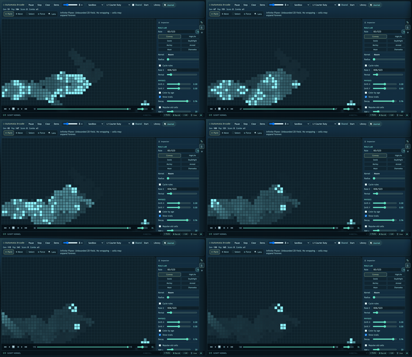
<figure class="wp-block-image alignwide size-large"><img data-recalc-dims="1" loading="lazy" decoding="async" width="960" height="540" data-attachment-id="1934" data-permalink="https://joelholder.com/2026/03/07/automata-arcade-building-a-playable-lab-for-conways-game-of-life/automata-arcade-demo/" data-orig-file="https://i0.wp.com/joelholder.com/wp-content/uploads/2026/03/automata-arcade-demo.gif?fit=960%2C540&amp;ssl=1" data-orig-size="960,540" data-comments-opened="1" data-image-meta="{&quot;aperture&quot;:&quot;0&quot;,&quot;credit&quot;:&quot;&quot;,&quot;camera&quot;:&quot;&quot;,&quot;caption&quot;:&quot;&quot;,&quot;created_timestamp&quot;:&quot;0&quot;,&quot;copyright&quot;:&quot;&quot;,&quot;focal_length&quot;:&quot;0&quot;,&quot;iso&quot;:&quot;0&quot;,&quot;shutter_speed&quot;:&quot;0&quot;,&quot;title&quot;:&quot;&quot;,&quot;orientation&quot;:&quot;0&quot;,&quot;alt&quot;:&quot;&quot;}" data-image-title="automata-arcade-demo" data-image-description="" data-image-caption="&lt;p&gt;Automata Arcade demo animation&lt;/p&gt;
" data-large-file="https://i0.wp.com/joelholder.com/wp-content/uploads/2026/03/automata-arcade-demo.gif?fit=960%2C540&amp;ssl=1" src="/assets/wp/automata-arcade-building-a-playable-lab-for-conways-game-of-life/automata-arcade-demo.gif" alt="Automata Arcade demo animation" class="wp-image-1934" /><figcaption>Automata Arcade demo animation</figcaption></figure>

<h3 class="wp-block-heading">Why this matters</h3>

<p class="wp-block-paragraph">Automata Arcade is a reminder that complex behavior can emerge from minimal rules, and that interactive systems can teach hard ideas quickly. Computation, resilience, failure modes, and control become tactile when you can build and intervene in real time.</p>

<p class="wp-block-paragraph">We are still early. There is far more power to unlock here.</p>]]></content><author><name>Joel Holder</name></author><summary type="html"><![CDATA[Automata Arcade turns Conway’s Game of Life into a live engineering arena. You do not just observe emergence, you shape it in real time.]]></summary></entry><entry><title type="html">Evo Lumen Life, creating a living ecosystem in the browser</title><link href="https://joelholder.com/blog/2026/03/02/evo-lumen-life-building-a-living-artificial-ecosystem-in-the-browser/" rel="alternate" type="text/html" title="Evo Lumen Life, creating a living ecosystem in the browser" /><published>2026-03-02T07:49:46+00:00</published><updated>2026-03-02T07:49:46+00:00</updated><id>https://joelholder.com/blog/2026/03/02/evo-lumen-life-building-a-living-artificial-ecosystem-in-the-browser</id><content type="html" xml:base="https://joelholder.com/blog/2026/03/02/evo-lumen-life-building-a-living-artificial-ecosystem-in-the-browser/"><![CDATA[<p class="wp-block-paragraph"><em>Evo Lumen Life</em> started as a shader experiment and became a living artificial-life sandbox where organisms swim, feed, reproduce, struggle, and evolve in a shared ecosystem.</p>

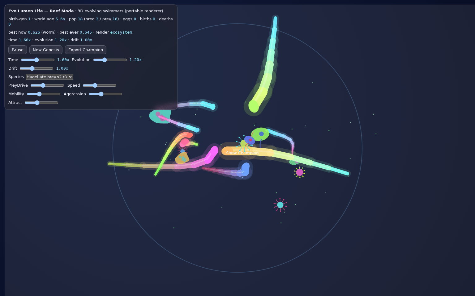
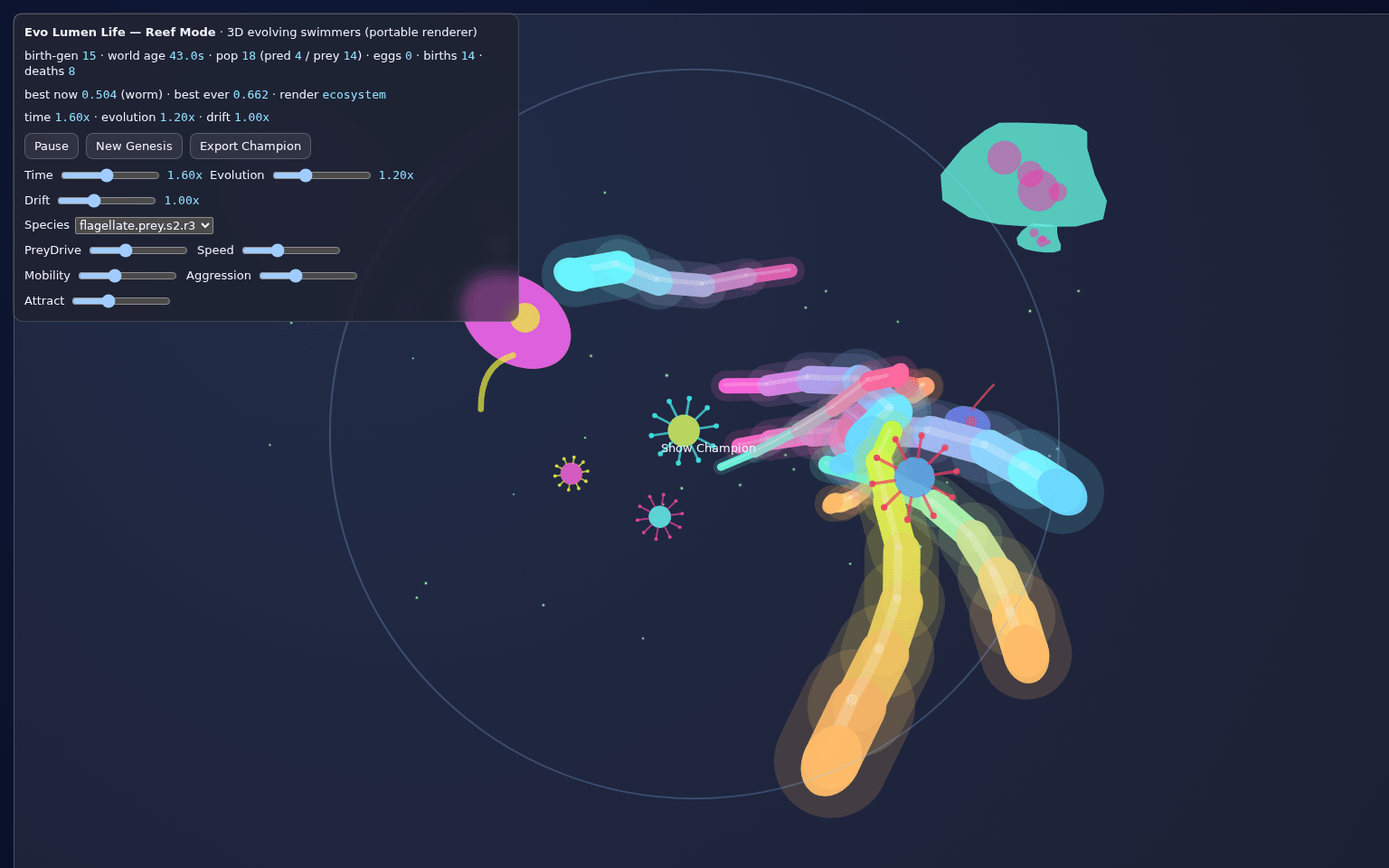
<p class="wp-block-paragraph"><strong>Project repo:</strong> <a href="https://github.com/jclosure/evo-lumen-life">https://github.com/jclosure/evo-lumen-life</a></p>

<h2 class="wp-block-heading">What it is</h2>

<p class="wp-block-paragraph">Evo Lumen Life is a browser-based simulation of emergent behavior. Instead of static entities, the world is populated by evolving forms (worms, flagellates, protozoa, and virus-like agents) whose movement and survival are shaped by local interaction rules, resource pressure, and reproduction strategies.</p>

<figure class="wp-block-image size-large"><img data-recalc-dims="1" decoding="async" src="/assets/wp/evo-lumen-life-building-a-living-artificial-ecosystem-in-the-browser/evo-overview-v2.png" alt="Evo Lumen Life ecosystem overview" /></figure>

<h2 class="wp-block-heading">Why?</h2>

<p class="wp-block-paragraph">I wanted something more alive than classic cellular automata: not just a pattern engine, but a watchable ecology. The design intent was to create a system that felt continuous and organic—something you could tune and observe like a tiny synthetic biosphere.</p>

<ul class="wp-block-list">
<li>Continuous lifecycle instead of abrupt generation resets</li>


<li>Predator/prey pressure and resource competition</li>


<li>Egg-based worm reproduction and juvenile growth</li>


<li>Interactive controls for time, evolution speed, drift, and species-level behavior</li>
</ul>

<h2 class="wp-block-heading">Goals</h2>

<ul class="wp-block-list">
<li><strong>Make emergence visible:</strong> behavior should unfold over time, not be hidden in static metrics.</li>


<li><strong>Keep it playful:</strong> enough complexity to surprise, enough controls to steer.</li>


<li><strong>Stay portable:</strong> run on Mac, Linux, and Windows in a browser.</li>


<li><strong>Favor flow:</strong> births, deaths, and adaptation drive the simulation</li>
</ul>

<figure class="wp-block-image size-large"><img data-recalc-dims="1" decoding="async" src="/assets/wp/evo-lumen-life-building-a-living-artificial-ecosystem-in-the-browser/evo-champion-view-v2.png" alt="Champion-focused view in Evo Lumen Life" /></figure>

<h2 class="wp-block-heading">What we learned</h2>

<p class="wp-block-paragraph">The strongest improvements came from treating the system as a controlled dynamical model and validating behavior under parameter sweeps.</p>

<ul class="wp-block-list">
<li><strong>State integration quality dominates perceived realism.</strong> We update organism state in small timesteps (position, velocity, energy, age), which reduces aliasing and prevents visual/mechanical discontinuities from coarse step changes.</li>


<li><strong>Bounded nonlinear terms are mandatory.</strong> Core drivers (aggression, drift, growth, resource intake) are clamped to stable ranges. Without bounds, positive feedback causes blow-up modes (population spikes, lock-step clumping, or immediate collapse).</li>


<li><strong>Energy economics creates meaningful behavior.</strong> A simple budget model (intake &#8211; metabolic cost &#8211; reproduction cost) produced emergent strategy differences more reliably than hand-scripted behavior trees.</li>


<li><strong>Asymmetry produces richer phase space.</strong> Predator-prey and forager-resource interactions are intentionally asymmetric; this increases attractor diversity versus symmetric pairwise rules.</li>


<li><strong>Fitness is multi-objective.</strong> Useful scoring required balancing persistence, exploration, locomotion efficiency, and survivability. Single-objective optimization collapsed diversity too quickly.</li>


<li><strong>Continuity constraints matter to observers.</strong> Interpolated hatch/growth curves and decay on death states improved interpretability and made causal chains easier to track.</li>


<li><strong>Live controls function as instrumentation.</strong> Real-time sliders effectively became online experiments: we could locate bifurcation-like regime shifts quickly and tune toward stable-but-interesting dynamics.</li>
</ul>

<p class="wp-block-paragraph">Bottom line: better outcomes came from numerical stability, bounded feedback, and measurable objective tradeoffs—not from adding more visual entities alone.</p>

<h2 class="wp-block-heading">Where this could go next</h2>

<ul class="wp-block-list">
<li>Speciation tracking with lineage trees and trait inheritance maps</li>


<li>Courtship and mate selection behaviors before egg-laying</li>


<li>Objective-driven environments (seasonality, gradients, hazards)</li>


<li>Replay/annotation mode for interesting events</li>


<li>Networked multiplayer ecosystem tournaments</li>


<li>Hybrid mode: AI ecology + human strategic interventions</li>
</ul>]]></content><author><name>Joel Holder</name></author><summary type="html"><![CDATA[Evo Lumen Life started as a shader experiment and became a living artificial-life sandbox where organisms swim, feed, reproduce, struggle, and evolve in a shared ecosystem.]]></summary></entry><entry><title type="html">Wrapping C and C++ APIs in Python</title><link href="https://joelholder.com/blog/2019/12/16/wrapping-c-apis-in-python/" rel="alternate" type="text/html" title="Wrapping C and C++ APIs in Python" /><published>2019-12-16T23:24:10+00:00</published><updated>2019-12-16T23:24:10+00:00</updated><id>https://joelholder.com/blog/2019/12/16/wrapping-c-apis-in-python</id><content type="html" xml:base="https://joelholder.com/blog/2019/12/16/wrapping-c-apis-in-python/"><![CDATA[<figure class="wp-block-image size-full"><img decoding="async" src="/assets/wp/wrapping-c-apis-in-python/python-cpp-hero.jpg" alt="Line-art illustration of Python and C++ working together at a laptop" /></figure>

<p class="wp-block-paragraph">Python is usually where I want to orchestrate work: load data, shape inputs, run experiments, and glue systems together. C and C++ are where I want hot loops, existing native libraries, SIMD-heavy routines, mature systems code, and APIs that already exist outside the Python ecosystem.</p>

<p class="wp-block-paragraph">The useful question is not whether Python or C is better. The useful question is where the boundary should be. If the native side has a small stable ABI, <code>ctypes</code> is often enough. If the boundary needs C++ types, exceptions, RAII, overloaded functions, or a clean Python-facing module, reach for <code>pybind11</code>.</p>

<h2 class="wp-block-heading">Start with the ABI</h2>

<p class="wp-block-paragraph">For a C API, the minimum viable path is:</p>

<ul class="wp-block-list"><li>build a shared library for the target platform</li><li>load it with <code>ctypes.CDLL</code></li><li>declare each function&#8217;s argument types and return type</li><li>be explicit about memory ownership and error behavior</li></ul>

<p class="wp-block-paragraph">Using <a href="https://github.com/simplegeo/libgeohash">libgeohash</a> as an example, a simple Linux build might look like this:</p>

<div class="language-bash highlighter-rouge"><div class="highlight"><pre class="highlight"><code>gcc <span class="nt">-O3</span> <span class="nt">-fPIC</span> <span class="nt">-shared</span> <span class="nt">-o</span> libgeohash.so geohash.c
</code></pre></div></div>

<p class="wp-block-paragraph">On macOS that output would usually be a <code>.dylib</code>; on Windows, a <code>.dll</code>. The Python code should not assume the extension unless you control deployment.</p>

<h2 class="wp-block-heading">A small ctypes wrapper</h2>

<p class="wp-block-paragraph">The important part of <code>ctypes</code> is not the load call. It is declaring the ABI accurately. Without <code>argtypes</code> and <code>restype</code>, Python will guess, and those guesses are not a contract you want in production.</p>

<div class="language-python highlighter-rouge"><div class="highlight"><pre class="highlight"><code><span class="kn">from</span> <span class="nn">ctypes</span> <span class="kn">import</span> <span class="n">CDLL</span><span class="p">,</span> <span class="n">c_char_p</span><span class="p">,</span> <span class="n">c_double</span><span class="p">,</span> <span class="n">c_int</span>
<span class="kn">from</span> <span class="nn">pathlib</span> <span class="kn">import</span> <span class="n">Path</span>

<span class="n">lib</span> <span class="o">=</span> <span class="n">CDLL</span><span class="p">(</span><span class="nb">str</span><span class="p">(</span><span class="n">Path</span><span class="p">(</span><span class="n">__file__</span><span class="p">).</span><span class="n">with_name</span><span class="p">(</span><span class="s">"libgeohash.so"</span><span class="p">)))</span>

<span class="k">def</span> <span class="nf">bind</span><span class="p">(</span><span class="n">name</span><span class="p">,</span> <span class="n">restype</span><span class="p">,</span> <span class="o">*</span><span class="n">argtypes</span><span class="p">):</span>
    <span class="n">fn</span> <span class="o">=</span> <span class="nb">getattr</span><span class="p">(</span><span class="n">lib</span><span class="p">,</span> <span class="n">name</span><span class="p">)</span>
    <span class="n">fn</span><span class="p">.</span><span class="n">restype</span> <span class="o">=</span> <span class="n">restype</span>
    <span class="n">fn</span><span class="p">.</span><span class="n">argtypes</span> <span class="o">=</span> <span class="nb">list</span><span class="p">(</span><span class="n">argtypes</span><span class="p">)</span>
    <span class="k">return</span> <span class="n">fn</span>

<span class="n">geohash_encode</span> <span class="o">=</span> <span class="n">bind</span><span class="p">(</span>
    <span class="s">"geohash_encode"</span><span class="p">,</span>
    <span class="n">c_char_p</span><span class="p">,</span>
    <span class="n">c_double</span><span class="p">,</span>
    <span class="n">c_double</span><span class="p">,</span>
    <span class="n">c_int</span><span class="p">,</span>
<span class="p">)</span>

<span class="n">raw</span> <span class="o">=</span> <span class="n">geohash_encode</span><span class="p">(</span><span class="mf">41.41845703125</span><span class="p">,</span> <span class="mf">2.17529296875</span><span class="p">,</span> <span class="mi">5</span><span class="p">)</span>
<span class="n">hash_value</span> <span class="o">=</span> <span class="n">raw</span><span class="p">.</span><span class="n">decode</span><span class="p">(</span><span class="s">"ascii"</span><span class="p">)</span>
<span class="k">print</span><span class="p">(</span><span class="n">hash_value</span><span class="p">)</span>  <span class="c1"># sp3e9
</span></code></pre></div></div>

<p class="wp-block-paragraph">That wrapper is intentionally boring. A Python call crosses into native code, the C function receives two doubles and an int, and the returned <code>char *</code> is exposed as bytes. The Python layer decodes it because the C ABI does not know about Python strings.</p>

<h2 class="wp-block-heading">Structs map cleanly when layout is simple</h2>

<p class="wp-block-paragraph">For plain C structs, define a matching <code>ctypes.Structure</code>. The order and C types must match the header. If the C side has packing pragmas, bitfields, platform-dependent integer sizes, or nested ownership, slow down and verify layout with tests.</p>

<div class="language-cpp highlighter-rouge"><div class="highlight"><pre class="highlight"><code><span class="k">typedef</span> <span class="k">struct</span> <span class="nc">GeoBoxDimensionStruct</span> <span class="p">{</span>
    <span class="kt">double</span> <span class="n">height</span><span class="p">;</span>
    <span class="kt">double</span> <span class="n">width</span><span class="p">;</span>
<span class="p">}</span> <span class="n">GeoBoxDimension</span><span class="p">;</span>

<span class="k">extern</span> <span class="n">GeoBoxDimension</span> <span class="n">geohash_dimensions_for_precision</span><span class="p">(</span><span class="kt">int</span> <span class="n">precision</span><span class="p">);</span>
</code></pre></div></div>

<div class="language-python highlighter-rouge"><div class="highlight"><pre class="highlight"><code><span class="kn">from</span> <span class="nn">ctypes</span> <span class="kn">import</span> <span class="n">Structure</span><span class="p">,</span> <span class="n">c_double</span><span class="p">,</span> <span class="n">c_int</span>

<span class="k">class</span> <span class="nc">GeoBoxDimension</span><span class="p">(</span><span class="n">Structure</span><span class="p">):</span>
    <span class="n">_fields_</span> <span class="o">=</span> <span class="p">[</span>
        <span class="p">(</span><span class="s">"height"</span><span class="p">,</span> <span class="n">c_double</span><span class="p">),</span>
        <span class="p">(</span><span class="s">"width"</span><span class="p">,</span> <span class="n">c_double</span><span class="p">),</span>
    <span class="p">]</span>

<span class="n">geohash_dimensions_for_precision</span> <span class="o">=</span> <span class="n">bind</span><span class="p">(</span>
    <span class="s">"geohash_dimensions_for_precision"</span><span class="p">,</span>
    <span class="n">GeoBoxDimension</span><span class="p">,</span>
    <span class="n">c_int</span><span class="p">,</span>
<span class="p">)</span>

<span class="n">dims</span> <span class="o">=</span> <span class="n">geohash_dimensions_for_precision</span><span class="p">(</span><span class="mi">6</span><span class="p">)</span>
<span class="k">print</span><span class="p">(</span><span class="n">dims</span><span class="p">.</span><span class="n">height</span><span class="p">,</span> <span class="n">dims</span><span class="p">.</span><span class="n">width</span><span class="p">)</span>
</code></pre></div></div>

<p class="wp-block-paragraph">This is a good shape for <code>ctypes</code>: value types cross the boundary, Python receives a small struct, and there is no lifecycle problem to solve.</p>

<h2 class="wp-block-heading">Out parameters and buffers</h2>

<p class="wp-block-paragraph">Many C APIs return status codes and write results through pointers. Model that directly. Do not pretend every C function is a Python function that returns one object.</p>

<div class="language-cpp highlighter-rouge"><div class="highlight"><pre class="highlight"><code><span class="kt">int</span> <span class="nf">geohash_decode_bbox</span><span class="p">(</span>
    <span class="k">const</span> <span class="kt">char</span> <span class="o">*</span><span class="n">hash</span><span class="p">,</span>
    <span class="kt">double</span> <span class="o">*</span><span class="n">lat_min</span><span class="p">,</span>
    <span class="kt">double</span> <span class="o">*</span><span class="n">lat_max</span><span class="p">,</span>
    <span class="kt">double</span> <span class="o">*</span><span class="n">lng_min</span><span class="p">,</span>
    <span class="kt">double</span> <span class="o">*</span><span class="n">lng_max</span>
<span class="p">);</span>
</code></pre></div></div>

<div class="language-python highlighter-rouge"><div class="highlight"><pre class="highlight"><code><span class="kn">from</span> <span class="nn">ctypes</span> <span class="kn">import</span> <span class="n">POINTER</span><span class="p">,</span> <span class="n">byref</span><span class="p">,</span> <span class="n">c_char_p</span><span class="p">,</span> <span class="n">c_double</span><span class="p">,</span> <span class="n">c_int</span>

<span class="n">geohash_decode_bbox</span> <span class="o">=</span> <span class="n">bind</span><span class="p">(</span>
    <span class="s">"geohash_decode_bbox"</span><span class="p">,</span>
    <span class="n">c_int</span><span class="p">,</span>
    <span class="n">c_char_p</span><span class="p">,</span>
    <span class="n">POINTER</span><span class="p">(</span><span class="n">c_double</span><span class="p">),</span>
    <span class="n">POINTER</span><span class="p">(</span><span class="n">c_double</span><span class="p">),</span>
    <span class="n">POINTER</span><span class="p">(</span><span class="n">c_double</span><span class="p">),</span>
    <span class="n">POINTER</span><span class="p">(</span><span class="n">c_double</span><span class="p">),</span>
<span class="p">)</span>

<span class="k">def</span> <span class="nf">decode_bbox</span><span class="p">(</span><span class="n">hash_value</span><span class="p">:</span> <span class="nb">str</span><span class="p">):</span>
    <span class="n">lat_min</span> <span class="o">=</span> <span class="n">c_double</span><span class="p">()</span>
    <span class="n">lat_max</span> <span class="o">=</span> <span class="n">c_double</span><span class="p">()</span>
    <span class="n">lng_min</span> <span class="o">=</span> <span class="n">c_double</span><span class="p">()</span>
    <span class="n">lng_max</span> <span class="o">=</span> <span class="n">c_double</span><span class="p">()</span>

    <span class="n">rc</span> <span class="o">=</span> <span class="n">geohash_decode_bbox</span><span class="p">(</span>
        <span class="n">hash_value</span><span class="p">.</span><span class="n">encode</span><span class="p">(</span><span class="s">"ascii"</span><span class="p">),</span>
        <span class="n">byref</span><span class="p">(</span><span class="n">lat_min</span><span class="p">),</span>
        <span class="n">byref</span><span class="p">(</span><span class="n">lat_max</span><span class="p">),</span>
        <span class="n">byref</span><span class="p">(</span><span class="n">lng_min</span><span class="p">),</span>
        <span class="n">byref</span><span class="p">(</span><span class="n">lng_max</span><span class="p">),</span>
    <span class="p">)</span>
    <span class="k">if</span> <span class="n">rc</span> <span class="o">!=</span> <span class="mi">0</span><span class="p">:</span>
        <span class="k">raise</span> <span class="nb">ValueError</span><span class="p">(</span><span class="sa">f</span><span class="s">"geohash_decode_bbox failed: </span><span class="si">{</span><span class="n">rc</span><span class="si">}</span><span class="s">"</span><span class="p">)</span>

    <span class="k">return</span> <span class="n">lat_min</span><span class="p">.</span><span class="n">value</span><span class="p">,</span> <span class="n">lat_max</span><span class="p">.</span><span class="n">value</span><span class="p">,</span> <span class="n">lng_min</span><span class="p">.</span><span class="n">value</span><span class="p">,</span> <span class="n">lng_max</span><span class="p">.</span><span class="n">value</span>
</code></pre></div></div>

<p class="wp-block-paragraph">The wrapper converts the C style into a Python style at the edge: allocate output slots, call the native function, check the return code, and return a tuple. That keeps the rest of the Python application free of pointer management.</p>

<h2 class="wp-block-heading">Use pybind11 when the boundary wants to be a module</h2>

<p class="wp-block-paragraph"><code>ctypes</code> works best against a C ABI. Once the native side is C++, or once you want a polished Python module instead of a thin ABI wrapper, <a href="https://github.com/pybind/pybind11">pybind11</a> is usually cleaner. You write a small C++ binding layer, compile it as a Python extension, and expose Python-native functions/classes.</p>

<div class="language-cpp highlighter-rouge"><div class="highlight"><pre class="highlight"><code><span class="c1">// bindings.cpp</span>
<span class="cp">#include</span> <span class="cpf">&lt;pybind11/pybind11.h&gt;</span><span class="cp">
#include</span> <span class="cpf">&lt;pybind11/stl.h&gt;</span><span class="cp">
#include</span> <span class="cpf">&lt;stdexcept&gt;</span><span class="cp">
#include</span> <span class="cpf">&lt;string&gt;</span><span class="cp">
</span>
<span class="k">namespace</span> <span class="n">py</span> <span class="o">=</span> <span class="n">pybind11</span><span class="p">;</span>

<span class="k">extern</span> <span class="s">"C"</span> <span class="kt">char</span> <span class="o">*</span><span class="nf">geohash_encode</span><span class="p">(</span><span class="kt">double</span> <span class="n">lat</span><span class="p">,</span> <span class="kt">double</span> <span class="n">lng</span><span class="p">,</span> <span class="kt">int</span> <span class="n">precision</span><span class="p">);</span>

<span class="k">struct</span> <span class="nc">Box</span> <span class="p">{</span>
    <span class="kt">double</span> <span class="n">height</span><span class="p">;</span>
    <span class="kt">double</span> <span class="n">width</span><span class="p">;</span>
<span class="p">};</span>

<span class="n">Box</span> <span class="n">dimensions_for_precision</span><span class="p">(</span><span class="kt">int</span> <span class="n">precision</span><span class="p">)</span> <span class="p">{</span>
    <span class="c1">// In real code this would call the native library.</span>
    <span class="k">return</span> <span class="n">Box</span><span class="p">{</span><span class="mf">0.0054931640625</span><span class="p">,</span> <span class="mf">0.010986328125</span><span class="p">};</span>
<span class="p">}</span>

<span class="n">std</span><span class="o">::</span><span class="n">string</span> <span class="n">encode</span><span class="p">(</span><span class="kt">double</span> <span class="n">lat</span><span class="p">,</span> <span class="kt">double</span> <span class="n">lng</span><span class="p">,</span> <span class="kt">int</span> <span class="n">precision</span><span class="p">)</span> <span class="p">{</span>
    <span class="kt">char</span> <span class="o">*</span><span class="n">raw</span> <span class="o">=</span> <span class="n">geohash_encode</span><span class="p">(</span><span class="n">lat</span><span class="p">,</span> <span class="n">lng</span><span class="p">,</span> <span class="n">precision</span><span class="p">);</span>
    <span class="k">if</span> <span class="p">(</span><span class="n">raw</span> <span class="o">==</span> <span class="nb">nullptr</span><span class="p">)</span> <span class="p">{</span>
        <span class="k">throw</span> <span class="n">std</span><span class="o">::</span><span class="n">runtime_error</span><span class="p">(</span><span class="s">"geohash_encode returned null"</span><span class="p">);</span>
    <span class="p">}</span>
    <span class="k">return</span> <span class="n">std</span><span class="o">::</span><span class="n">string</span><span class="p">(</span><span class="n">raw</span><span class="p">);</span>
<span class="p">}</span>

<span class="n">PYBIND11_MODULE</span><span class="p">(</span><span class="n">geohash_native</span><span class="p">,</span> <span class="n">m</span><span class="p">)</span> <span class="p">{</span>
    <span class="n">m</span><span class="p">.</span><span class="n">doc</span><span class="p">()</span> <span class="o">=</span> <span class="s">"Native geohash bindings"</span><span class="p">;</span>

    <span class="n">py</span><span class="o">::</span><span class="n">class_</span><span class="o">&lt;</span><span class="n">Box</span><span class="o">&gt;</span><span class="p">(</span><span class="n">m</span><span class="p">,</span> <span class="s">"Box"</span><span class="p">)</span>
        <span class="p">.</span><span class="n">def_readonly</span><span class="p">(</span><span class="s">"height"</span><span class="p">,</span> <span class="o">&amp;</span><span class="n">Box</span><span class="o">::</span><span class="n">height</span><span class="p">)</span>
        <span class="p">.</span><span class="n">def_readonly</span><span class="p">(</span><span class="s">"width"</span><span class="p">,</span> <span class="o">&amp;</span><span class="n">Box</span><span class="o">::</span><span class="n">width</span><span class="p">);</span>

    <span class="n">m</span><span class="p">.</span><span class="n">def</span><span class="p">(</span><span class="s">"encode"</span><span class="p">,</span> <span class="o">&amp;</span><span class="n">encode</span><span class="p">,</span>
        <span class="n">py</span><span class="o">::</span><span class="n">arg</span><span class="p">(</span><span class="s">"lat"</span><span class="p">),</span>
        <span class="n">py</span><span class="o">::</span><span class="n">arg</span><span class="p">(</span><span class="s">"lng"</span><span class="p">),</span>
        <span class="n">py</span><span class="o">::</span><span class="n">arg</span><span class="p">(</span><span class="s">"precision"</span><span class="p">)</span> <span class="o">=</span> <span class="mi">12</span><span class="p">);</span>

    <span class="n">m</span><span class="p">.</span><span class="n">def</span><span class="p">(</span><span class="s">"dimensions_for_precision"</span><span class="p">,</span> <span class="o">&amp;</span><span class="n">dimensions_for_precision</span><span class="p">);</span>
<span class="p">}</span>
</code></pre></div></div>

<p class="wp-block-paragraph">A minimal build using <code>setuptools</code> can stay small:</p>

<div class="language-python highlighter-rouge"><div class="highlight"><pre class="highlight"><code><span class="c1"># setup.py
</span><span class="kn">from</span> <span class="nn">pybind11.setup_helpers</span> <span class="kn">import</span> <span class="n">Pybind11Extension</span><span class="p">,</span> <span class="n">build_ext</span>
<span class="kn">from</span> <span class="nn">setuptools</span> <span class="kn">import</span> <span class="n">setup</span>

<span class="n">ext_modules</span> <span class="o">=</span> <span class="p">[</span>
    <span class="n">Pybind11Extension</span><span class="p">(</span>
        <span class="s">"geohash_native"</span><span class="p">,</span>
        <span class="p">[</span><span class="s">"bindings.cpp"</span><span class="p">,</span> <span class="s">"geohash.c"</span><span class="p">],</span>
        <span class="n">cxx_std</span><span class="o">=</span><span class="mi">17</span><span class="p">,</span>
    <span class="p">),</span>
<span class="p">]</span>

<span class="n">setup</span><span class="p">(</span>
    <span class="n">name</span><span class="o">=</span><span class="s">"geohash_native"</span><span class="p">,</span>
    <span class="n">ext_modules</span><span class="o">=</span><span class="n">ext_modules</span><span class="p">,</span>
    <span class="n">cmdclass</span><span class="o">=</span><span class="p">{</span><span class="s">"build_ext"</span><span class="p">:</span> <span class="n">build_ext</span><span class="p">},</span>
<span class="p">)</span>
</code></pre></div></div>

<div class="language-bash highlighter-rouge"><div class="highlight"><pre class="highlight"><code>python <span class="nt">-m</span> pip <span class="nb">install </span>pybind11 setuptools wheel
python <span class="nt">-m</span> pip <span class="nb">install</span> <span class="nt">-e</span> <span class="nb">.</span>
</code></pre></div></div>

<div class="language-python highlighter-rouge"><div class="highlight"><pre class="highlight"><code><span class="kn">import</span> <span class="nn">geohash_native</span>

<span class="k">print</span><span class="p">(</span><span class="n">geohash_native</span><span class="p">.</span><span class="n">encode</span><span class="p">(</span><span class="mf">41.41845703125</span><span class="p">,</span> <span class="mf">2.17529296875</span><span class="p">,</span> <span class="n">precision</span><span class="o">=</span><span class="mi">5</span><span class="p">))</span>

<span class="n">box</span> <span class="o">=</span> <span class="n">geohash_native</span><span class="p">.</span><span class="n">dimensions_for_precision</span><span class="p">(</span><span class="mi">6</span><span class="p">)</span>
<span class="k">print</span><span class="p">(</span><span class="n">box</span><span class="p">.</span><span class="n">height</span><span class="p">,</span> <span class="n">box</span><span class="p">.</span><span class="n">width</span><span class="p">)</span>
</code></pre></div></div>

<p class="wp-block-paragraph">The tradeoff is build complexity. With <code>ctypes</code>, Python loads an existing shared object. With <code>pybind11</code>, you ship a compiled Python extension for each supported Python/platform/architecture combination. The upside is a nicer API, better C++ interop, and fewer pointer-shaped details leaking into application code.</p>

<h2 class="wp-block-heading">Rules of thumb</h2>

<ul class="wp-block-list"><li>Use <code>ctypes</code> when the native library already exposes a stable C ABI and the surface area is small.</li><li>Use <code>pybind11</code> when you own the native code, need C++ types, or want a Pythonic module.</li><li>Keep allocation and freeing on the same side of the boundary unless the API explicitly documents otherwise.</li><li>Turn C status codes into Python exceptions at the wrapper edge.</li><li>Write tests for struct layout, null pointers, invalid inputs, and at least one known-good result from the native library.</li><li>Benchmark the boundary. Crossing into native code is cheap enough for coarse operations, but not something to do once per scalar in a Python loop.</li></ul>

<p class="wp-block-paragraph">The clean version is simple: keep Python in charge of orchestration, keep native code responsible for the expensive or already-existing work, and make the boundary explicit. A thin wrapper is often enough, but the moment the boundary becomes part of your product API, give it the same design attention as any other public interface.</p>]]></content><author><name>Joel Holder</name></author><category term="C#" /><category term="Interop" /><category term="Python" /><category term="Speed" /><summary type="html"><![CDATA[]]></summary></entry><entry><title type="html">EventBusBridges for Great Good</title><link href="https://joelholder.com/blog/2016/06/19/eventbusbridges-for-great-good/" rel="alternate" type="text/html" title="EventBusBridges for Great Good" /><published>2016-06-19T07:09:22+00:00</published><updated>2016-06-19T07:09:22+00:00</updated><id>https://joelholder.com/blog/2016/06/19/eventbusbridges-for-great-good</id><content type="html" xml:base="https://joelholder.com/blog/2016/06/19/eventbusbridges-for-great-good/"><![CDATA[<p>The <a href="http://sockjs.org">SockJS protocol</a> provides a fast and reliable mechanism for providing duplex communication via Websockets. Vertx has a particularly nice implementation of this in the form of <a href="http://vertx.io/docs/vertx-web/java/#_handling_event_bus_bridge_events">EventBusBridges</a>, which make it easy to create secure communication pipelines between an HttpServer Verticle and a variety of polyglot SockJS clients via Websockets or fallback transports. Surprisingly, a Java-based EventBusBridgeClient is not among the ootb facilities, even though Java is the main story on the server. Here I will show you how easy to create your own and a few of the awesome things you can do with it.</p>

<h4 id="the-eventbusbridge-server">The EventBusBridge Server</h4>

<div class="language-java highlighter-rouge"><div class="highlight"><pre class="highlight"><code><span class="nc">Router</span> <span class="n">router</span> <span class="o">=</span> <span class="nc">Router</span><span class="o">.</span><span class="na">router</span><span class="o">(</span><span class="n">vertx</span><span class="o">);</span>

<span class="c1">// Allow all addresses to flow in and out on the bridge</span>

<span class="nc">BridgeOptions</span> <span class="n">options</span> <span class="o">=</span> <span class="k">new</span> <span class="nc">BridgeOptions</span><span class="o">()</span>
  <span class="o">.</span><span class="na">addInboundPermitted</span><span class="o">(</span><span class="k">new</span> <span class="nc">PermittedOptions</span><span class="o">().</span><span class="na">setAddressRegex</span><span class="o">(</span><span class="s">".+"</span><span class="o">))</span>
  <span class="o">.</span><span class="na">addOutboundPermitted</span><span class="o">(</span><span class="k">new</span> <span class="nc">PermittedOptions</span><span class="o">().</span><span class="na">setAddressRegex</span><span class="o">(</span><span class="s">".+"</span><span class="o">));</span>

<span class="n">router</span><span class="o">.</span><span class="na">route</span><span class="o">(</span><span class="s">"/eventbus/*"</span><span class="o">).</span><span class="na">handler</span><span class="o">(</span>
  <span class="nc">SockJSHandler</span><span class="o">.</span><span class="na">create</span><span class="o">(</span><span class="n">vertx</span><span class="o">).</span><span class="na">bridge</span><span class="o">(</span><span class="n">options</span><span class="o">)</span>
<span class="o">);</span>

<span class="c1">// Setup a body handler</span>
<span class="n">router</span><span class="o">.</span><span class="na">route</span><span class="o">().</span><span class="na">handler</span><span class="o">(</span><span class="nc">BodyHandler</span><span class="o">.</span><span class="na">create</span><span class="o">());</span>

<span class="nc">HttpServer</span> <span class="n">httpServer</span> <span class="o">=</span> <span class="n">vertx</span><span class="o">.</span><span class="na">createHttpServer</span><span class="o">();</span>
<span class="n">httpServer</span><span class="o">.</span><span class="na">requestHandler</span><span class="o">(</span><span class="nl">router:</span><span class="o">:</span><span class="n">accept</span><span class="o">).</span><span class="na">listen</span><span class="o">(</span><span class="mi">8080</span><span class="o">);</span>

<span class="c1">// do server wiring</span>

<span class="c1">// Publish a message to "someaddress" on interval</span>
<span class="n">vertx</span><span class="o">.</span><span class="na">setPeriodic</span><span class="o">(</span><span class="mi">5000</span><span class="o">,</span> <span class="n">t</span> <span class="o">-&gt;</span> <span class="o">{</span>
  <span class="nc">JsonObject</span> <span class="n">msg</span> <span class="o">=</span> <span class="k">new</span> <span class="nc">JsonObject</span><span class="o">().</span><span class="na">put</span><span class="o">(</span><span class="s">"packet"</span><span class="o">,</span> <span class="s">"stuff"</span><span class="o">);</span>
  <span class="n">vertx</span><span class="o">.</span><span class="na">eventBus</span><span class="o">().</span><span class="na">publish</span><span class="o">(</span><span class="s">"someaddress"</span><span class="o">,</span> <span class="n">msg</span><span class="o">);</span>
<span class="o">});</span>

<span class="c1">// Consume messages the "importantstuff" address</span>
<span class="n">vertx</span><span class="o">.</span><span class="na">eventBus</span><span class="o">().</span><span class="na">consumer</span><span class="o">(</span><span class="s">"importantstuff"</span><span class="o">,</span> <span class="n">msg</span> <span class="o">-&gt;</span> <span class="o">{</span>
  <span class="n">logger</span><span class="o">.</span><span class="na">warn</span><span class="o">(</span><span class="n">msg</span><span class="o">.</span><span class="na">body</span><span class="o">());</span>
<span class="o">});</span>
</code></pre></div></div>

<p>With this server code we are extending the EventBus via a Websocket. It’s available to <a href="https://github.com/sockjs/sockjs-client">any client</a> that can speak the SockJS protocol. We can also easily write a Java client that will speak the SockJS-protocol to our server.</p>

<h4 id="the-java-sockjs-client">The Java SockJS Client</h4>

<div class="language-java highlighter-rouge"><div class="highlight"><pre class="highlight"><code><span class="kd">private</span> <span class="kd">static</span> <span class="kd">final</span> <span class="nc">String</span> <span class="n">pingMessage</span><span class="o">;</span>

<span class="kd">static</span> <span class="o">{</span>
  <span class="nc">JsonObject</span> <span class="n">json</span> <span class="o">=</span> <span class="k">new</span> <span class="nc">JsonObject</span><span class="o">();</span>
  <span class="n">json</span><span class="o">.</span><span class="na">put</span><span class="o">(</span><span class="s">"type"</span><span class="o">,</span> <span class="s">"ping"</span><span class="o">);</span>
  <span class="n">pingMessage</span> <span class="o">=</span> <span class="n">json</span><span class="o">.</span><span class="na">encode</span><span class="o">();</span>
<span class="o">}</span>

<span class="nc">HttpClient</span> <span class="n">client</span> <span class="o">=</span> <span class="n">vertx</span><span class="o">.</span><span class="na">createHttpClient</span><span class="o">();</span>

<span class="c1">// We use raw websocket transport</span>
<span class="n">client</span><span class="o">.</span><span class="na">websocket</span><span class="o">(</span><span class="n">port</span><span class="o">,</span> <span class="n">host</span><span class="o">,</span> <span class="s">"/eventbus/websocket"</span><span class="o">,</span> <span class="n">websocket</span> <span class="o">-&gt;</span> <span class="o">{</span>

<span class="c1">// Register</span>
<span class="nc">JsonObject</span> <span class="n">msg</span> <span class="o">=</span> <span class="k">new</span> <span class="nc">JsonObject</span><span class="o">().</span><span class="na">put</span><span class="o">(</span><span class="s">"type"</span><span class="o">,</span> <span class="s">"register"</span><span class="o">).</span><span class="na">put</span><span class="o">(</span>
  <span class="s">"address"</span><span class="o">,</span> <span class="s">"someaddress"</span>
<span class="o">);</span>
<span class="n">websocket</span><span class="o">.</span><span class="na">writeFinalTextFrame</span><span class="o">(</span><span class="n">msg</span><span class="o">.</span><span class="na">encode</span><span class="o">());</span>

<span class="c1">// Setup pinging for keepalive</span>
<span class="n">pingTimerId</span> <span class="o">=</span> <span class="nc">Vertx</span><span class="o">.</span><span class="na">currentContext</span><span class="o">().</span><span class="na">owner</span><span class="o">().</span><span class="na">setPeriodic</span><span class="o">(</span>
  <span class="mi">5000</span><span class="o">,</span> <span class="n">event</span> <span class="o">-&gt;</span> <span class="o">{</span>
    <span class="n">websocket</span><span class="o">.</span><span class="na">writeFinalTextFrame</span><span class="o">(</span><span class="n">pingMessage</span><span class="o">);</span>
  <span class="o">}</span>
<span class="o">);</span>

<span class="c1">// Send to the server</span>
<span class="n">msg</span> <span class="o">=</span> <span class="k">new</span> <span class="nc">JsonObject</span><span class="o">().</span><span class="na">put</span><span class="o">(</span><span class="s">"type"</span><span class="o">,</span> <span class="s">"send"</span><span class="o">)</span>
<span class="o">.</span><span class="na">put</span><span class="o">(</span><span class="s">"address"</span><span class="o">,</span> <span class="s">"importantstuff"</span><span class="o">)</span>
<span class="o">.</span><span class="na">put</span><span class="o">(</span><span class="s">"body"</span><span class="o">,</span> <span class="k">new</span> <span class="nc">JsonObject</span><span class="o">().</span><span class="na">put</span><span class="o">(</span><span class="s">"foo"</span><span class="o">,</span> <span class="s">"bar"</span><span class="o">));</span>
<span class="n">websocket</span><span class="o">.</span><span class="na">writeFinalTextFrame</span><span class="o">(</span><span class="n">msg</span><span class="o">.</span><span class="na">encode</span><span class="o">());</span>

<span class="c1">// Receive from the server</span>
<span class="n">websocket</span><span class="o">.</span><span class="na">handler</span><span class="o">(</span><span class="n">buffer</span> <span class="o">-&gt;</span> <span class="o">{</span>
  <span class="nc">JsonObject</span> <span class="n">received</span> <span class="o">=</span> <span class="k">new</span> <span class="nc">JsonObject</span><span class="o">(</span><span class="n">buffer</span><span class="o">.</span><span class="na">toString</span><span class="o">());</span>

  <span class="n">logger</span><span class="o">.</span><span class="na">info</span><span class="o">(</span>
    <span class="s">"received message on address: "</span> <span class="o">+</span> <span class="n">received</span><span class="o">.</span><span class="na">getString</span><span class="o">(</span><span class="s">"address"</span><span class="o">)</span>
  <span class="o">);</span>
  <span class="n">logger</span><span class="o">.</span><span class="na">info</span><span class="o">(</span><span class="s">"message body: "</span> <span class="o">+</span> <span class="n">received</span><span class="o">.</span><span class="na">getString</span><span class="o">(</span><span class="s">"body"</span><span class="o">));</span>
  <span class="o">});</span>
<span class="o">});</span>
</code></pre></div></div>

<p>Note that first we must “register” the client with the server. This is accomplished by sending a properly crafted register message, which is just a json packet with the type set to “register” along with the address the client wants to subscribe to. Additionally, the SockJS protocol specifies a “ping” message for keep alive on the socket. We provide a properly crafted pingMessage to enable this at the top of this code.</p>

<p>The envelope for SockJS messages is specified in the protocol to look like this:</p>

<div class="language-javascript highlighter-rouge"><div class="highlight"><pre class="highlight"><code><span class="p">{</span>
<span class="dl">"</span><span class="s2">type</span><span class="dl">"</span><span class="p">:</span> <span class="dl">"</span><span class="s2">send</span><span class="dl">"</span><span class="o">|</span><span class="dl">"</span><span class="s2">publish</span><span class="dl">"</span><span class="o">|</span><span class="dl">"</span><span class="s2">receive</span><span class="dl">"</span><span class="o">|</span><span class="dl">"</span><span class="s2">register</span><span class="dl">"</span><span class="o">|</span><span class="dl">"</span><span class="s2">unregister</span><span class="dl">"</span><span class="p">,</span>
<span class="dl">"</span><span class="s2">address</span><span class="dl">"</span><span class="p">:</span> <span class="dl">"</span><span class="s2">mailbox123</span><span class="dl">"</span>
<span class="dl">"</span><span class="s2">body</span><span class="dl">"</span><span class="p">:</span> <span class="dl">"</span><span class="s2">the body of the message</span><span class="dl">"</span>
<span class="p">}</span>
</code></pre></div></div>

<p>You can see in the client implementation above we performed a “send” by specifying it in the JsonObject envelope.</p>

<p>The operations specified by the protocol are these:</p>

<p><strong>SOCKET_CREATED</strong>
This event will occur when a new SockJS socket is created.</p>

<p><strong>SOCKET_CLOSED</strong>
This event will occur when a SockJS socket is closed.</p>

<p><strong>SEND</strong>
This event will occur when a message is attempted to be sent from the client to the server.</p>

<p><strong>PUBLISH</strong>
This event will occur when a message is attempted to be published from the client to the server.</p>

<p><strong>RECEIVE</strong>
This event will occur when a message is attempted to be delivered from the server to the client.</p>

<p><strong>REGISTER</strong>
This event will occur when a client attempts to register a handler.</p>

<p><strong>UNREGISTER</strong>
This event will occur when a client attempts to unregister a handler.</p>

<p>You can see how trivial relaying to a proxied address or republishing on a local EventBus might be by simply switching over these operations. In the kinds of patterns this substrates enables, you can see in things like <a href="http://www.enterpriseintegrationpatterns.com/patterns/messaging/PointToPointChannel.html">Point-to-Point Channel</a>, <a href="http://www.enterpriseintegrationpatterns.com/patterns/messaging/PublishSubscribeChannel.html">Publish-Subscribe Channel</a>, and <a href="http://www.enterpriseintegrationpatterns.com/patterns/messaging/BroadcastAggregate.html">Scatter-Gather</a> messaging.</p>

<p>The Javascript sockjs-client can be found <a href="https://github.com/sockjs/sockjs-client">here</a>. Vertx includes an eventbus-client, <a href="https://github.com/vert-x3/vertx-examples/blob/master/web-examples/src/main/java/io/vertx/example/web/realtime/webroot/vertx-eventbus.js">vertx-eventbus.js</a>, that utilizes sockjs.js to provide a convenient extension of the EventBus into Javascript apps. This is ideal for running in the browser, bolting realtime messaging directly into your web apps. There is also an <a href="https://www.npmjs.com/package/vertx3-eventbus-client">npm module</a> that brings allows you to easily snap node apps into your eventing framework. Someone has even recently created a <a href="https://github.com/julien3/vertxbuspp">C++ implementation</a> that provides an onramp to your native runtime applications.</p>

<p>This is a fantastically powerful composition medium. I highly recommend it as the foundation for modern, high-speed, real-time software that needs to start small but scale to immense sizes. Thanks to Vertx, its just cake.</p>

<p>Enjoy the cake…</p>]]></content><author><name>Joel Holder</name></author><summary type="html"><![CDATA[The SockJS protocol provides a fast and reliable mechanism for providing duplex communication via Websockets. Vertx has a particularly nice implementation of this in the form of EventBusBridges, which make it easy to create secure communication pipelines between an HttpServer Verticle and a variety of polyglot SockJS clients via Websockets or fallback transports. Surprisingly, a Java-based EventBusBridgeClient is not among the ootb facilities, even though Java is the main story on the server. Here I will show you how easy to create your own and a few of the awesome things you can do with it.]]></summary></entry></feed>